Chapter 13 Transformations
We have seen previously that we must check residuals carefully to make sure the assumptions of our linear model are valid.
The following example should be clear. Let us suppose we are measuring the number of bacteria (y) in a dish after it has been left unwashed for a certain number of hours (x).
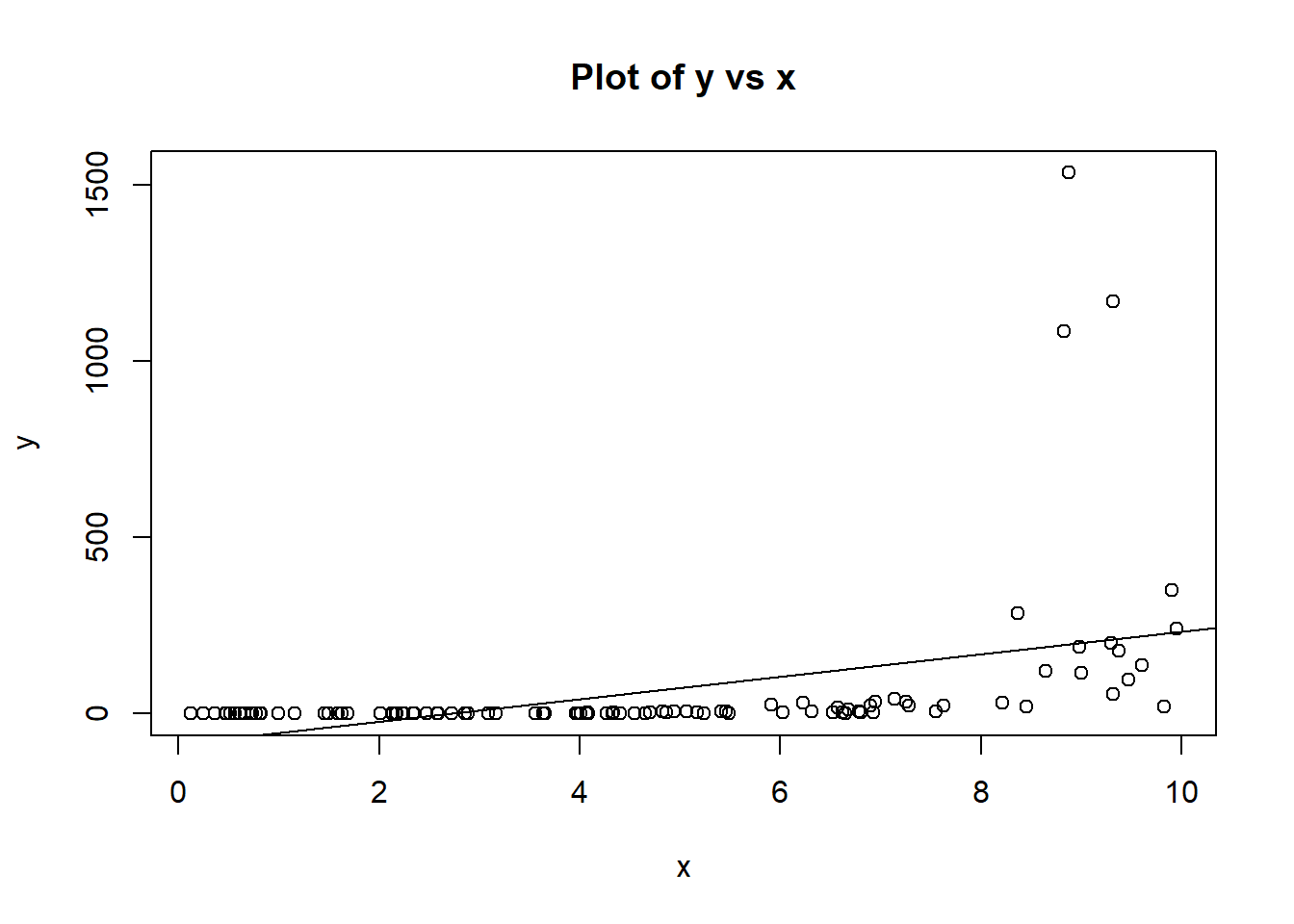
Our first thought might be to plot the raw data, and plot the linear model.
plot(x,y,main = "Plot of y vs x")
abline(lm(y~x))
plot(lm(y~x),which=1)
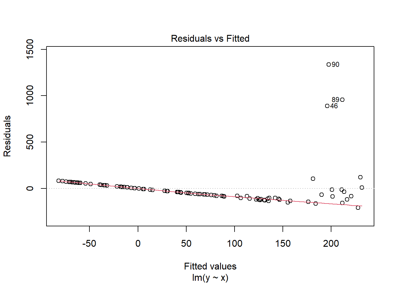
Clearly we can see that the linear model does not fit; we can see this both on the plot of the raw data, but note especially the funnel shape in the residual plot; the variance of the residuals is small on the left, but large on the right. This breaks our model assumptions, which imply that our residuals have the same variance for any fitted value of y.
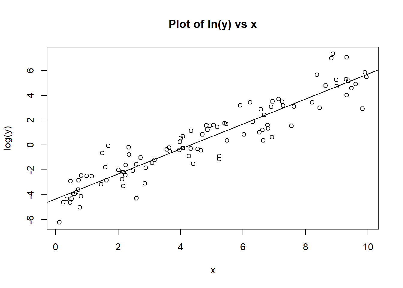
There is no reason that y and x should be linear, so an easy fix in this case might be a transformation, where we plot log(y) against x.
plot(x,log(y),main = "Plot of ln(y) vs x")
abline(lm(log(y)~x))
plot(lm(log(y)~x),which=1)
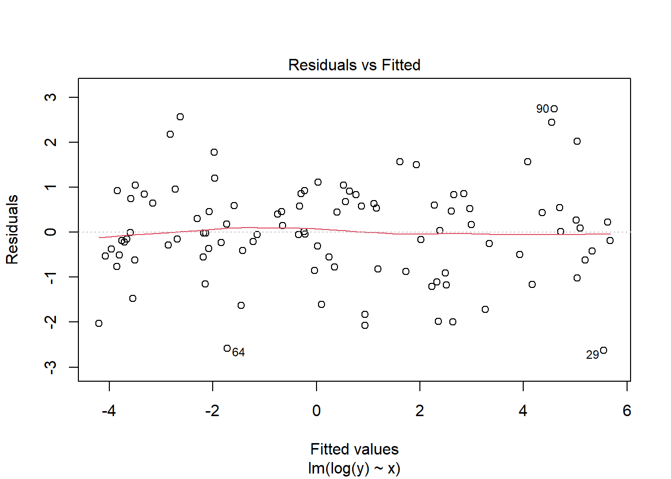
Here we see a much happier plot of log(y) against x, which shows potential for a linear relationship, and we can see from the residual plot that our “funnel shape” in our residuals has disappeared.
In this chapter, you will go through examples to allow you to get familiar with using R when our linear model does not fit.
13.1 Using transformations- The Restaurant Data
We consider the extent to which the valuation of a restaurant is determined by its sales figures: is there a relationship between sales and valuation? Can sales be used to predict valuation? We will use simple linear regression but find that we need to transform variables to obtain an acceptable model.
The data we use are part of a larger study, where many variables were recorded for a sample of 279 Wisconsin restaurants. The data are available in the file restrnt.txt. We can read this into R as follows
rest <- read.table("https://www.dropbox.com/s/igq343a4tefdqo1/restrnt.txt?dl=1", header=T)In this analysis, we are interested in the variables SALES and VALUE, both of which are recorded in thousands of dollars. Note that 9 restaurants have a valuation of 0 which, for the purposes on this analysis, we will assume to represent a missing value. We perform this data recoding by
rest$VALUE[rest$VALUE==0] <- NA- Obtain summary statistics for the data columns
SALESandVALUE. As there are missing values, (denoted in the data frame by NA), some summary calculations (for examplemean) by default assume that missing values should be ignored, but we can make this explicit, for examplemean(rest$SALES, na.rm=T). - Plot
VALUEagainstSALES, making sure the axes have informative labels and the graph an informative title. This plot is difficult to interpret and we see a linear relationship cannot be justified. -It is informative to fit a simple linear regression model (the response isVALUEand the explanatory variableSALESand look at the residual plots to see how they indicate the inappropriateness of this model; do this here to see what they look like. - We will need to transform the variables to better satisfy the model assumptions. When transforming data, is is common to consider a logarithmic transformation of the response variable, or of both the response and explanatory variables. Try
plot(rest$SALES, log(rest$VALUE))
plot(log(rest$SALES), log(rest$VALUE))- You should see that the latter transformation seems as if it might make simple linear regression a plausible model, so fit a simple linear regression with
log(VALUE)as the response andlog(SALES)as the explanatory variable. This can be achieved by creating new transformed variables in the data frame and then fitting the linear model as
##
## Call:
## lm(formula = log(VALUE) ~ log(SALES), data = rest)
##
## Residuals:
##     Min      1Q  Median      3Q     Max
## -3.8045 -0.4275  0.0974  0.4489  2.0945
##
## Coefficients:
##             Estimate Std. Error t value Pr(>|t|)
## (Intercept)   1.1157     0.2664   4.188 4.04e-05 ***
## log(SALES)    0.7785     0.0500  15.570  < 2e-16 ***
## ---
## Signif. codes:  0 '***' 0.001 '**' 0.01 '*' 0.05 '.' 0.1 ' ' 1
##
## Residual standard error: 0.7933 on 224 degrees of freedom
##   (53 observations deleted due to missingness)
## Multiple R-squared:  0.5198, Adjusted R-squared:  0.5176
## F-statistic: 242.4 on 1 and 224 DF, p-value: < 2.2e-16- Use residual plots to check the model assumptions for this log-log transformed model. While we might still not be entirely satisfied looking at the diagnostic plots, they are much better than before applying the transformation.
- What does this linear model imply for the relationship between the original (transformed) variables, VALUE and SALES? is the relationship linear on the original scale? Write down an equation you might use to predict VALUE form SALES (note that, in R, the function
logcomputes natural logarithms, by default). - So far we have only added one term to the model. Using the techniques we learnt last week for linear modelling, can you add more terms to improve the model further?
- We have used log as our transformation, but in general (although there are some techniques to help) knowing which transformation will work is a case of some educated guessing. Do different transformations (e.g. \(1/y\)) help improve the model?
suppressPackageStartupMessages({
  library(tidyverse)   # loading ggplot2 and dplyr
})