Chapter 6 Inference

A main theme of statistics is inference: using some information from a sample to find out something about the population the sample has come from. For example, we ask 100 randomly chosen people whether they support a proposition that children should be given milk at school, and 37 of them agree. What can we say about the proportion of people that agree with the proposition across the entire region? How sure can we be about any statement we make? This general procedure is called inference.

We first introduce the Central Limit Theorem, before we talk about forming Confidence Intervals.

6.1 The Central Limit Theoerem

The Central Limit Theorem says that, given a sufficiently large sample size from a population, the mean of all samples from the same population will be approximately equal to the mean of the original population. It also says that as we increase the number of samples and the sample size, the distribution of all of the sample means will become approximately Normal — irrespective of what the population distribution is. This distribution is referred to as the sampling distribution.

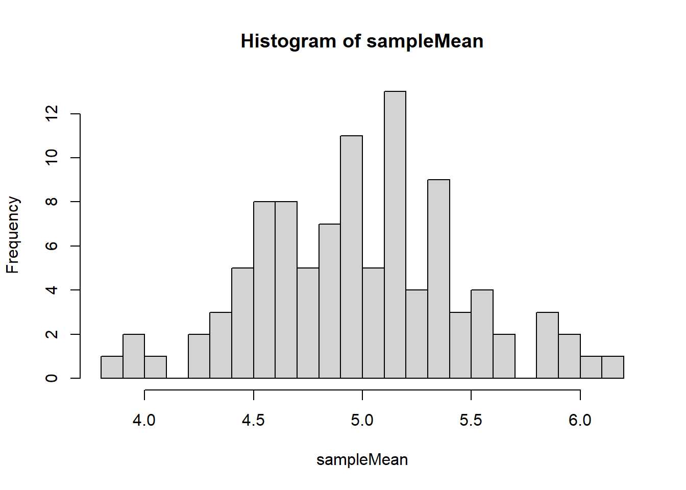
Let’s try to demonstrate this using R, putting together the coding that we have learnt so far. Imagine we run an experiment where we have 100 events that can either happen (success) or non happen (fail) each with probability 0.05, which we pretend is not known. We pretend that we can run this experiment 20 times, and for each run we record the number of successes, out of 100. Based on these 20 runs, we wish to guess the true unknown probability.

Formally, we’re going to take a sample, samp of size m=20 from a Binomial(100,0.05) distribution, and record the sample mean, mean(samp). We’re going to do this s=100 times, and look at the distribution of the sample mean: the sampling distribution.

popSize <- 100   # Number of trials (population size)
p<- 0.05 # Population Probability of "success"

s <- 100 # Number of simulations
m <- 20 #sampleSize    

sampleMean<-c(0) # Set the vector to be zero initially 
for (i in 1:s){
    samp <- rbinom(n = m, size = popSize, prob = 0.05)
    sampleMean[i] <- mean(samp) # sample mean
}

hist(sampleMean,breaks = 25)

Try changing the values of s , the number of simulations, and m, the sample size. You should see that increasing either makes the distribution look more like a Gaussian distribution.

There is a nice https://gallery.shinyapps.io/CLT_mean/ which demonstrates the Central Limit theorem in an easy to use format. Shiny is a way of building web apps for R which allows the user to interact, and this is a good demo of slightly more advanced uses of R.

6.2 Confidence Intervals

Suppose we’ve collected a random sample of 12 people; we ask them to run for 100m and record their heart rate afterwards

Imagine that this is the data we see:

##  [1]  94.39524  97.69823 115.58708 100.70508 101.29288 117.15065 104.60916  87.34939
##  [9]  93.13147  95.54338 112.24082 103.59814

We want to estimate the mean heart rate after exercise for our population (i.e. not just people in our sample), and form a 90% and 95% confidence interval for the mean.

6.2.1 Known variance/standard deviation

Assume that heart rates are normally distributed with unknown mean and standard deviation \(\sigma=10\).

## Warning: package 'gghighlight' was built under R version 4.1.3

## Warning: Using `across()` in `filter()` is deprecated, use `if_any()` or `if_all()`.

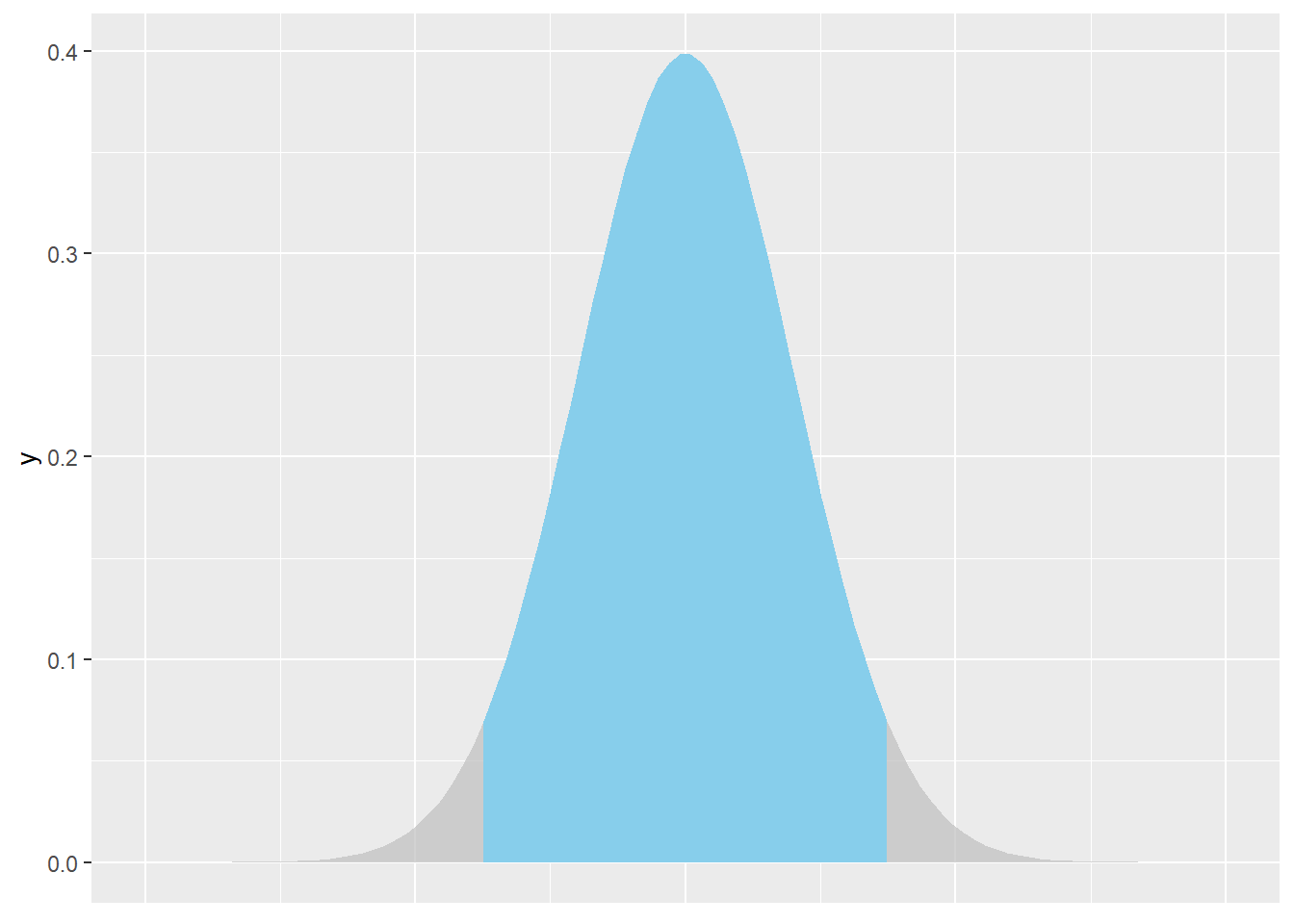
We wish to find the central area shaded blue, i.e. an area that corresponds to a range of values in which the true mean is likely to lie based on our sample data. If this area represents 90% of the distribution, this is called a 90% Confidence interval. Note for a 90% confidence interval, the grey areas in each tail would each represent 5%.

We know from theory that a \((1-\alpha)100\%\) Confidence Interval is given by \[\bar{X}\pm z_{\frac{\alpha}{2}}\frac{\sigma}{\sqrt{n}}\] We know n = 12, and are given \(\sigma = 10\).

For a 90% confidence interval, we get \(\alpha=0.10\), and we can calculate \(z_{\frac{\alpha}{2}}=z_{0.05}\) from R:

qnorm(.95)

## [1] 1.644854

qnorm(.05)

## [1] -1.644854

And the sample mean is just:

mean(x)

## [1] 101.9418

Thus our lower and upper bounds are

lb<-mean(x)-qnorm(0.95)*(10/sqrt(12))
ub<-mean(x)+qnorm(0.95)*(10/sqrt(12))
c(lb,ub)

## [1]  97.19351 106.69008

Thus our confidence interval can be written as (97.19,106.69).

Change the value of 0.95 above to see what happens for a 95% confidence interval. Is it narrower or wider than a 90% confidence interval?

6.2.2 Unknown Variance/Standard Deviation.

Let us assume that we do not know the standard deviation. We must now estimate it from the data

sd(x)

## [1] 9.253206

When the variance is unknown, we can no longer use the normal distribution, but must use an appropriate t-distribution, in this case with \(n-1\) degrees of freedom. Our CI is now given by \[\bar{X}\pm t_{n-1,\frac{\alpha}{2}}\frac{s}{\sqrt{n}}\] where \(s\) is the sample standard deviation

We can calculate the 90% percentile for the t-distribution:

qt(.95,df = 11)

## [1] 1.795885

Putting it all together means if we do not know the variance, then lower and upper bounds are

lb<-mean(x)-qt(.95,df = 11)*(sd(x)/sqrt(12))
ub<-mean(x)+qt(.95,df = 11)*(sd(x)/sqrt(12))
c(lb, ub)

## [1]  97.14468 106.73891

Thus our 90% confidence interval can be written as (97.14,106.74).

How does this compare to the CI with the variance assumed known? Again, can you change this to find a 95% confidence interval?

6.3 Interpretation of Confidence Intervals

We’re going to use a for loop generate 100 confidence intervals. We generate drawing \(n=10\) samples from a normal random variable, with mean 50, and standard deviation 5.

lb<-c(0) # initialise lb as a zero vector
ub<-c(0) # initialise ub as a zero vector
for (i in 1:100){
x<-rnorm(10,mean=50,sd=5)  
lb[i]<-mean(x)-qt(.95,df = 9)*(sd(x)/sqrt(10))
ub[i]<-mean(x)+qt(.95,df = 9)*(sd(x)/sqrt(10))
}

We’re going to add the lower and upper bounds to a data frame, and add a third column which is an indicator as to whether the confidence interval contains the true value of the mean, which is 50.

ci<-data.frame(lb,ub)
ci$coverage<-((lb<50)&(ub>50))
head(ci)

##         lb       ub coverage
## 1 46.60980 52.60673     TRUE
## 2 45.87350 51.29810     TRUE
## 3 49.33325 52.85318     TRUE
## 4 47.46825 53.57199     TRUE
## 5 48.36490 53.50450     TRUE
## 6 45.79179 52.76153     TRUE

A confidence interval for the mean is based on a sample, and gives us a range where we would expect the true value of the unknown mean to lie, based on the data. A 90% CI means that we would expect the CI to contain the true mean 90% of the time. Another way of saying that is that if we form 100 Confidence intervals from data taken from the same distribution, 90 of them would be expected to contain the true value (in this case 50).

We can see the number in this case as

sum(ci$coverage)

## [1] 91

Try repeating the generation of the 100 confidence intervals. How often do you get exactly 90? (Note this percentage of CIs that get the right result is known as the coverage.)

6.3.1 An animation

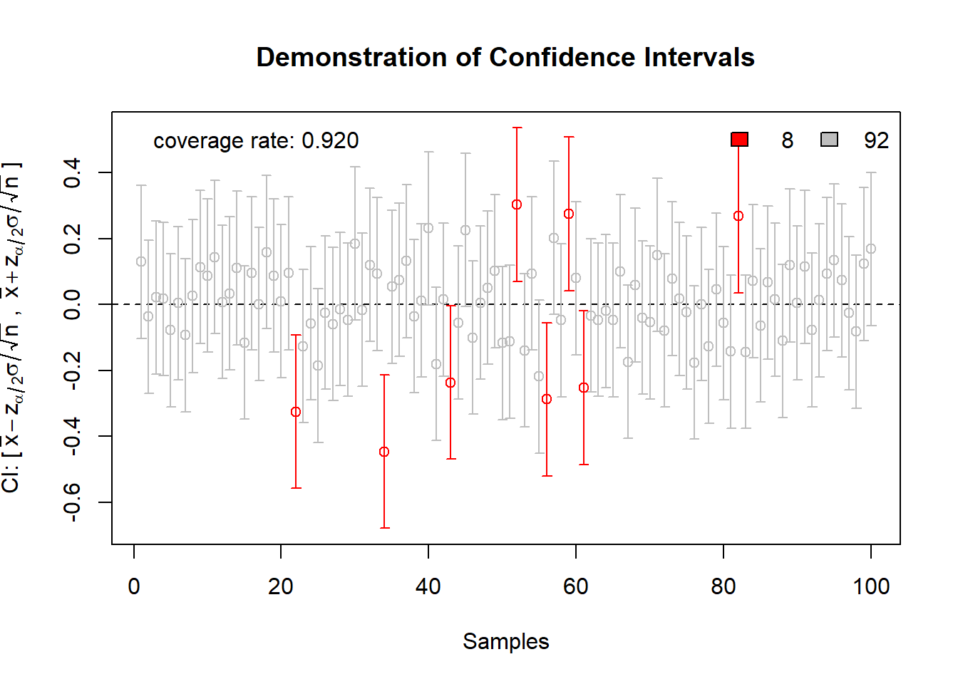
The animation package in R can nicely shows how confidence intervals are obtained. The following will draw 100 samples of size 50 from a \(N(0,1)\) distribution, and form a CI, highlighting whether or not the true mean of zero is found.

#install.packages("animation")
library(animation)
ani.options(interval = 0.1, nmax = 100)
conf.int(0.9, size=50, main = "Demonstration of Confidence Intervals")

This animation shows us clearly that every time we gather a new sample, we have a new CI. Because the CIs are random (they depend on the random sample), each CI we gather may or may not contain the mean. In the long term, for a 90% CI, approximately 90% of confidence intervals formed using this sampling procedure contain the true mean. Note this is not the same as saying that for a particular confidence interval, the probability that the true mean is in this range is 90%.

Exercises

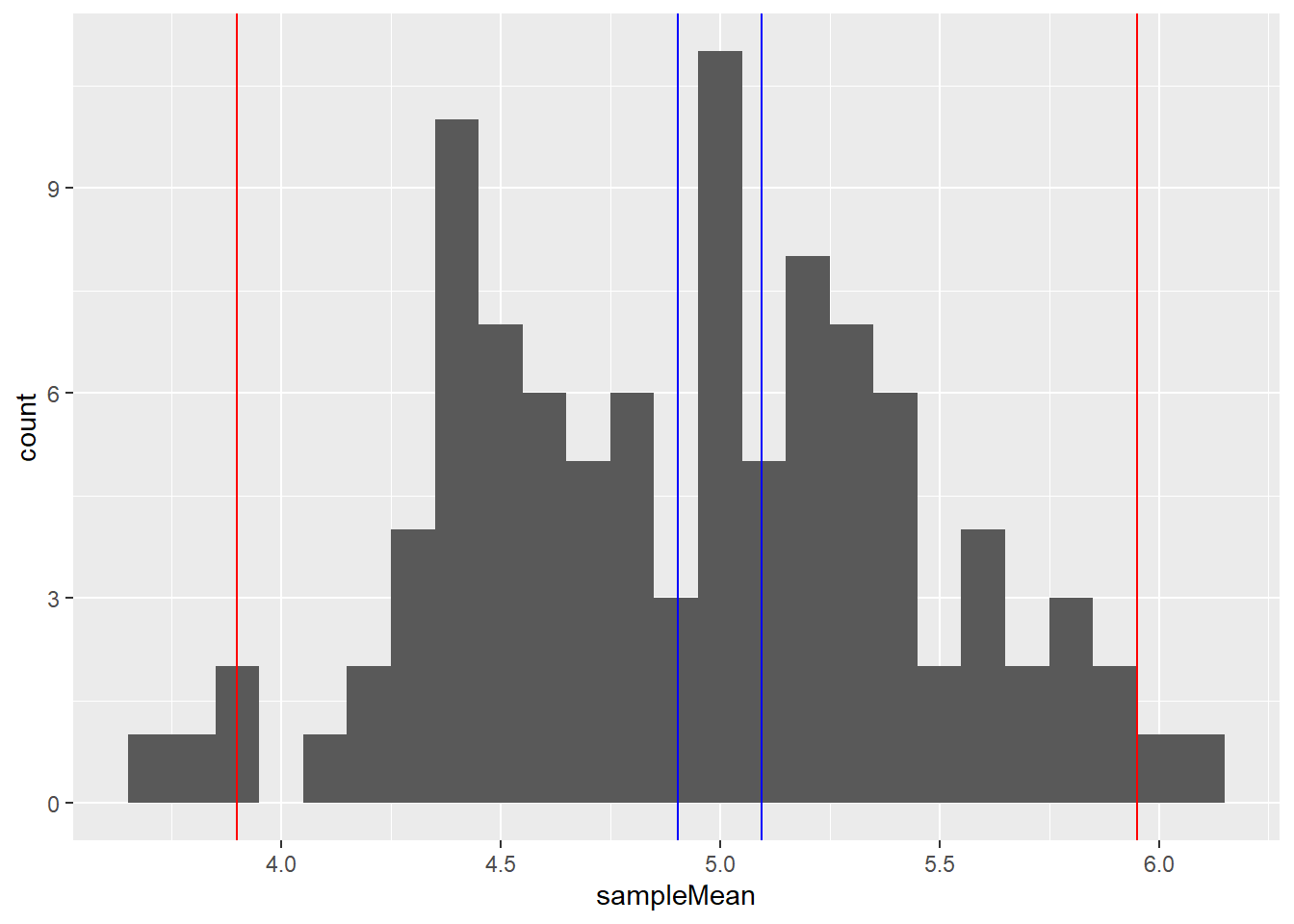
1. For the histogram demonstrating the central limit theorem from the Binomial(100,0.05) distribution, put two red vertical lines on the plot to indicate where the value that 95% of the sampleMean vector lie between. Hint: To add a vertical line in a plot, use the vline command, for example vline(v=2,col="red") will add a red line through x=2. To find the quantiles of a distribution (the value that a percentage of the data lies below) use the quantile command.
2. Generate in blue where the true confidence interval should be based on this data. Hint: what is the mean and variance of a binomial distribution with mean \(n\) and probability of success \(p\)? What therefore is the sample mean and sample variance?.

Repeat the exercise on forming the histogram for the central limit theorem, but change the distribution from a binomial(100,0.05) to
1. A Poisson distribution with parameter \(\mu=5\)
2. An exponential distribution with parameter \(\lambda=5\) One of these is a discrete distribution, one is a continuous distribution. Does the same general result hold?
The built in data set iris containts a variable Petal.Length. Assuming that the data was chosen at random (it almost certainly was not!), find a 95% CI for the mean Petal length for the distribution.