Chapter 12 Outliers and prediction
We have looked quite a lot at residual plots, but now let’s look a little deeper. A standardised residual is just the raw value of a residual divided by it’s (estimated) variance, formally defined as \[d_i = \frac{e_i}{\sqrt{s^2 (1-\frac{1}{n} + \frac{(x_i - \bar{x})^2}{S_{xx}})}}.\]
As these residuals are now standardised, we expect almost all residuals to lie within three standard deviations of zero, so if we see a standardised residual with an absolute value greater then 3 then it is an unusual observation, and we call this an outlier.
Outliers may be caused by a problem with the experiment, for example the measurement procedure is wrong or data has been mis-recorded. Care should be taken with unusual observations to establish whether they are genuine or not.
It may be that the reason we have an outlier is that our model does not fit; so if we detect an outlier we can either
- conclude that the data is a mistake, or that the observation is in some way not wanted in our model, and leave it out
- re-fit the model so that the standardised residuals are acceptable.
12.1 Influential observations
It may be that, even though an observation is unusual, including it does not alter the model substantially. There are two principle ways of assessing the influence of a point:
- The leverage of an observation measures the influence of the observation \(y_i\) on its own predicted value \(\hat{y_i}\). As a rule of thumb, the leverage is high if it is greater than \(2p/n\), where \(p\) is the number of parameters in the model, and \(n\) the number of data points.
- The Cook’s distance measures the effect of observation \(y_i\) on the estimated coefficients \(\hat{\beta_0}\), \(\hat{\beta_1}\), etc. We can perform a statistical test (actually an F test with p and n-p degrees of freedom) to see if it is influential.
12.1.1 Example- Fishy Data?
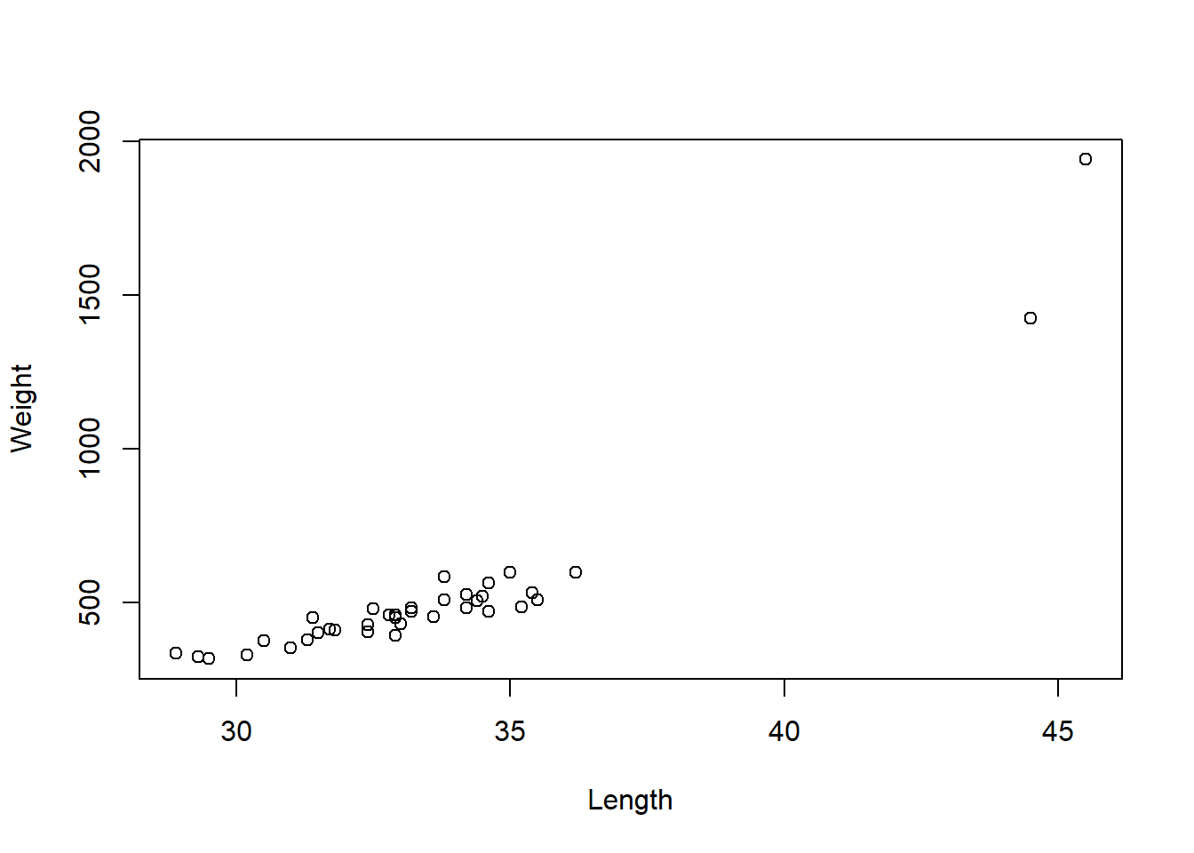
The file fish.txt contains the lengths and weights of 37 different fish. How can we find a model relating the length and the weight of a fish. In the simple linear model, are there any unusual observations? We first plot the data and look at the first residual plot from the linear model
fish<- read.table("https://www.dropbox.com/s/eu4eko0qmcu88wk/fish.txt?dl=1",header=TRUE)
plot(fish$length,fish$weight, xlab="Length", ylab="Weight")
fish.lm<-lm(weight~length,data=fish)
summary(fish.lm)
##
## Call:
## lm(formula = weight ~ length, data = fish)
##
## Residuals:
## Min 1Q Median 3Q Max
## -174.65 -74.28 -12.14 42.84 427.04
##
## Coefficients:
## Estimate Std. Error t value Pr(>|t|)
## (Intercept) -2254.839 195.845 -11.51 1.87e-13 ***
## length 82.831 5.815 14.24 3.92e-16 ***
## ---
## Signif. codes: 0 '***' 0.001 '**' 0.01 '*' 0.05 '.' 0.1 ' ' 1
##
## Residual standard error: 115.7 on 35 degrees of freedom
## Multiple R-squared: 0.8529, Adjusted R-squared: 0.8487
## F-statistic: 202.9 on 1 and 35 DF, p-value: 3.917e-16We could run a plot(fish.lm) to see all residual plots, or we can see more relevant residual plots by doing the following in R:
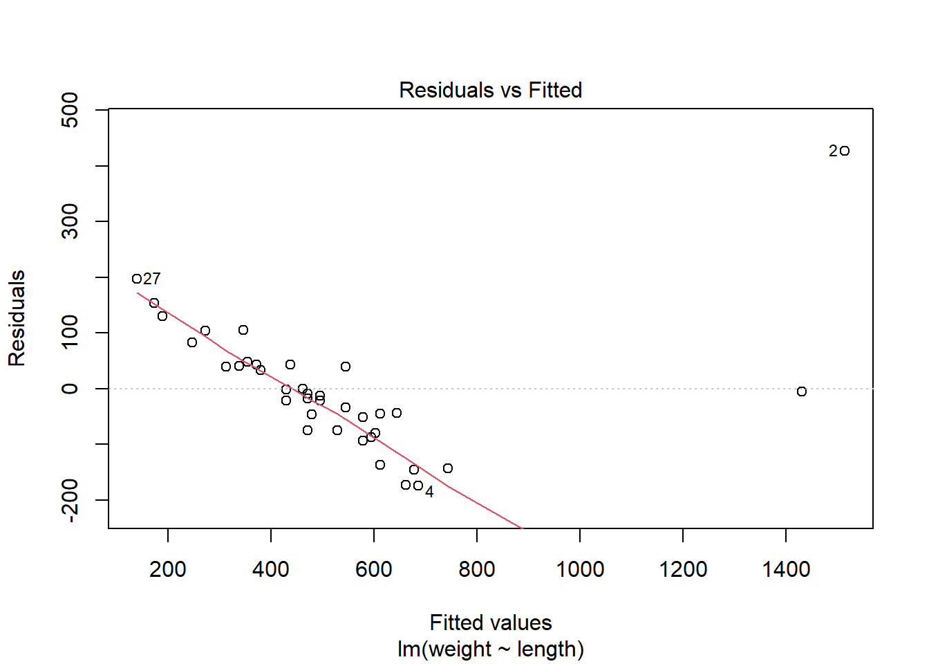
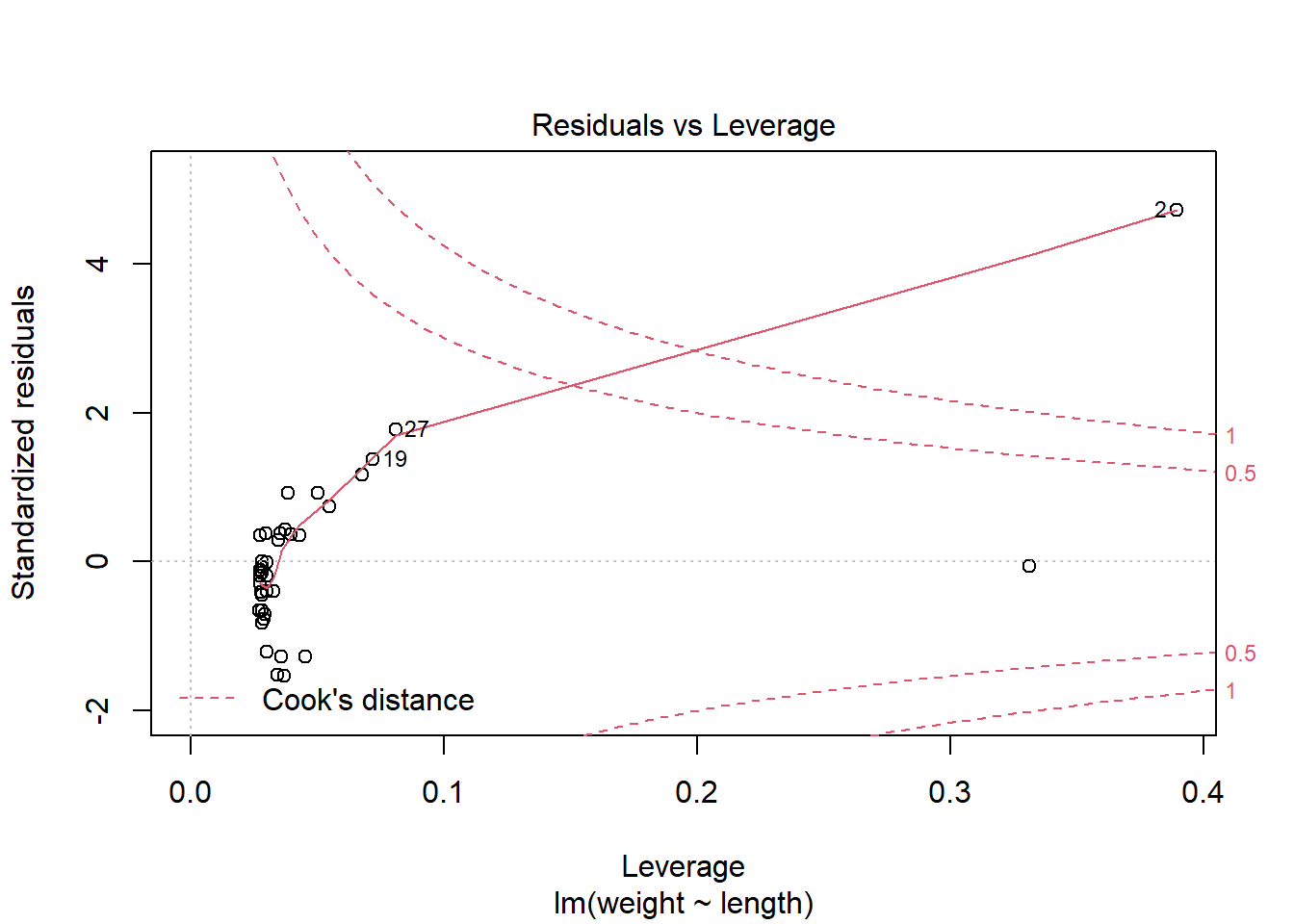
plot(fish.lm,which=c(5,1))

R labels the residuals which might be questionable- here 2, 4, and 27. Looking at the residuals, we see that R point 2 especially- with length 45.5 and weight 1941, the largest weight- is unusual. It has both a high Cook’s distance and a high value of leverage, which indicates that this point is very influential in the model.
We cannot conclude that this is necessary an incorrect reading; it is quite possible this is just a very large fish. If there is a problem, we can re-fit the model without point 2.
If there is no reason to question the data point, then we must find a model that does fit the data better.
12.1.2 Exercise
Continue the work on the fishy data set
- Remove the outlier with the largest standardised residual if it is
above 3. This is easiest in R by forming a new data frame, e.g.
fish <- fish[-5,] to remove the fifth row in the data frame. Does
removing this change the model substantially?
- Keep repeating this if necessary until you have a model which has no
outliers. Do you prefer the original model or the final model. Why?
- You may want to remove the point with the biggest influence (e.g.
Cook’s distance) first, then refit the model and possibly remove
further pointss. Do your conclusions change? Is this a sensible
procedure?
12.2 Prediction
We can use R to predict from our regression models as well- what would
happen if we have new data points. For example, looking back at our
simple linear regression model for the faithful data set, what would
we predict if we had a new observation waiting time.
### Prediction intervals
attach(faithful)
eruption.lm<-lm(eruptions~waiting)
predict(eruption.lm,data.frame(waiting=80),interval="prediction")
## fit lwr upr
## 1 4.17622 3.196089 5.156351R gives us the “fit” value, which is the point estimate for the new response at waiting time 80, and also gives a 95% prediction interval, which is a range of values which the new point may lie in.
We can do the same thing for multiple regression, for example for the executive salary dataset we looked at in the last chapter
exec<-read.table("https://www.dropbox.com/s/jefnudvc130xhzp/EXECSAL2.txt?dl=1",header=TRUE)
slm1<-lm(Y~X1+X3,data=exec)
newSal<-predict(slm1,data.frame(X1=12,X3=1),interval="prediction")
newSal
## fit lwr upr
## 1 11.49261 11.22971 11.7555Remember that this gives the logarithm of the salary! We can find the salary by:
exp(newSal)## fit lwr upr
## 1 97988.48 75335.8 127452.612.2.1 Exercises
- For the fish dataset, with the full data for the simple linear model:
- what is the predicted weight for a fish of length 30?
- what is the predicted weight for a fish of length 35?
- what are the prediction interevals for these two weights?
- how do these change if the one or two potential outliers are removed?
- For the execsal dataset in the last chapter, find the predicted salary for an executive with 10 years of experience, 14 years education, who is male, supervises 120 employees and with corporate asses of 150 million USD. Is the salary predicted to be lower if the executive were female?
suppressPackageStartupMessages({
  library(tidyverse)   # loading ggplot2 and dplyr
})