Chapter 14 Generalized Linear modelling
The Generalized Linear Model allows us to fit a much wider type of models than the linear models we have studied so far.
We will not go through the theory here (see this chapter as a brief tasty introduction to a much wider field), but essentially remember that our linear model was
\[Y_i=\beta_0+\beta_1x_{1i}+\beta_2x_{2i}+\ldots+\beta_{p-1}x_{p-1,i}+\epsilon_i\]
and we made some assumptions about the \(\epsilon_i\), usually that they were normal, independent, and identically distributed, with mean 0 and fixed variance \(\sigma^2\).
With the generalized model, we just assume that there is some model where we transform both the mean of the responses \(\mathbf{Y}\), and the errors, \(\mathbf{\epsilon}\) such that we end up with a model that is linear.
To be slightly more formal: The generalised linear model(GLM) is made up of linear predictor \[\nu_i=\beta_0+\beta_1x_{1i}+\beta_2x_{2i}+\ldots+\beta_{p-1}x_{p-1,i}+\epsilon_i\]
together with
- a link function that describes how the mean \(E(Y_i)=\mu_i\) ,is related to the linear predictor \(g(\mu_i)=\nu_i\)
- a variance function that describes how the variance \(\mbox{var}(Y_i)\) depends on the mean \(\mbox{var}(Y_i)=\phi V(\mu)\), where the dispersion parameter \(\phi\) is a constant.
14.1 Logistic Regression
In the logistic regression case, we have a resposne which is binary (either 0 or 1). Often, this is the chances of something happenning or not happening.
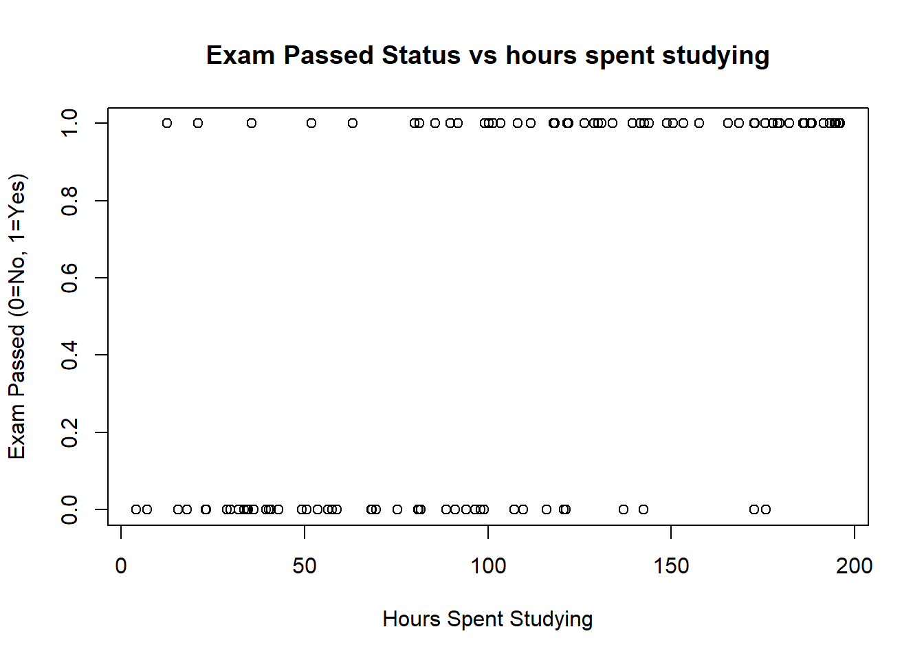
For example, consider the dataset where x is the number of hours spent studying for an exam, and y is whether the exam is passed. Clearly we would expect the probability of the exam being passed to relate to how long is spent studying, but perhaps there are other factors, including luck, to consider as well.
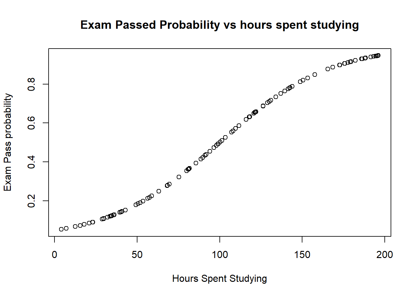
- The first plot above shows how the probability of passing changes with hour studying. Note we see a classic sigmoid (s shape): the passs probability tends towards zero with a low number of hours studying, and to 1 as lots of hours are spent studying.
- The second plot shows the results for the test against hours spent studying. Note that it is possible for students who spent little time studying to pass, as study time is likely to be one of only many factors that determine pass rate, and the other factors are not included in our model.
- Our model formally is that
\[log\left(\frac{p_i}{1-p_i}\right)=\beta_0+\beta_1x_i+\epsilon_i\] where \(p_i\) is the probability of passing, and \(x_i\) is the hours spent studying for student \(i\). We make the same assumptions about \(\epsilon_i\) as before in our simple linear model. The term \[log\left(\frac{p_i}{1-p_i}\right)\] is known as the logistic (or logit) transform.
14.1.1 Getting into Graduate School
The dataset binary.csv contains data on the chances of admission to US Graduate School.
We are interested in how GRE (Graduate Record Exam scores), GPA (grade point average) and prestige of the undergraduate institution (rated from 1 to 4, highest prestige to lowest prestige), affect admission into graduate school. The response variable is a binary variable, 0 for don’t admit, and 1 for admit.
The task is to find a model which relates the response to the regressor variables.
First read the data in and start to examine it with the following commands.
graduate <- read.csv("https://www.dropbox.com/s/pncohfbllms54ki/binary.csv?dl=1")
head(graduate)
## admit gre gpa rank
## 1 0 380 3.61 3
## 2 1 660 3.67 3
## 3 1 800 4.00 1
## 4 1 640 3.19 4
## 5 0 520 2.93 4
## 6 1 760 3.00 2summary(graduate)## admit gre gpa rank
## Min. :0.0000 Min. :220.0 Min. :2.260 Min. :1.000
## 1st Qu.:0.0000 1st Qu.:520.0 1st Qu.:3.130 1st Qu.:2.000
## Median :0.0000 Median :580.0 Median :3.395 Median :2.000
## Mean :0.3175 Mean :587.7 Mean :3.390 Mean :2.485
## 3rd Qu.:1.0000 3rd Qu.:660.0 3rd Qu.:3.670 3rd Qu.:3.000
## Max. :1.0000 Max. :800.0 Max. :4.000 Max. :4.000- As the response is binary, a natural first step is to try logistic regression. We must first tell R that rank is a categorical variable. (For example,we must tell R that rank=2 is not twice as big as rank=1)
graduate$rank <- factor(graduate$rank)
graduate.glm <- glm(admit ~ gre + gpa + rank, data = graduate,
                                          family = "binomial")
summary(graduate.glm)
##
## Call:
## glm(formula = admit ~ gre + gpa + rank, family = "binomial",
## data = graduate)
##
## Deviance Residuals:
## Min 1Q Median 3Q Max
## -1.6268 -0.8662 -0.6388 1.1490 2.0790
##
## Coefficients:
## Estimate Std. Error z value Pr(>|z|)
## (Intercept) -3.989979 1.139951 -3.500 0.000465 ***
## gre 0.002264 0.001094 2.070 0.038465 *
## gpa 0.804038 0.331819 2.423 0.015388 *
## rank2 -0.675443 0.316490 -2.134 0.032829 *
## rank3 -1.340204 0.345306 -3.881 0.000104 ***
## rank4 -1.551464 0.417832 -3.713 0.000205 ***
## ---
## Signif. codes: 0 '***' 0.001 '**' 0.01 '*' 0.05 '.' 0.1 ' ' 1
##
## (Dispersion parameter for binomial family taken to be 1)
##
## Null deviance: 499.98 on 399 degrees of freedom
## Residual deviance: 458.52 on 394 degrees of freedom
## AIC: 470.52
##
## Number of Fisher Scoring iterations: 4You should see that all the terms are significant, as well as some information about the deviance and the AIC. We define the log odds of an event A as \[\mbox{logit}(A)=\log\left(\frac{P(A)}{1-P(A)}\right).\]
The logistic regression coefficients in the R output give the change in the log odds of the outcome for a one unit increase in the predictor variable. For example, for a one unit increase in GPA, the log odds of being admitted to graduate school increases by 0.804.
As rank is a factor (categorical variable) the coefficients for rank have a slightly different interpretation. For example, having attended an undergraduate institution with rank of 2, versus an institution with a rank of 1, changes the log odds of admission by -0.675.
- Use the command
exp(coef(graduate.glm))to get the odds ratios. This will tell you, for example, that a one point increase in GRE increase the admission chances by a factor of 1.0023. - Use this model to predict the probability of admission for a student with GRE 700, GPA 3.7, to a rank 2 institution. To do this using R, we must first make a data frame
predData <- with(graduate, data.frame(gre = 700, gpa = 3.7, rank = factor(2)))
predData$prediction <- predict(graduate.glm, newdata = predData,
                                              type = "response")
predData
## gre gpa rank prediction
## 1 700 3.7 2 0.4736781Use the
confint(graduate.glm)command to get a confidence interval for the coefficients. These are based on the full profile of the log-likelihood function. We can also use theconfint.defaultcommand to just use the standard errors (i.e. assume that the confidence interval has a t distribution)We can check how well our model fits. We already saw that R produced a value for the AIC, which we can use to compare models. Earlier in the course we used an F test to check whether the fit of the overall model was significant for a linear model. Similarly, for a GLM, we can perfom a chi-squared test on the difference between the null deviance and the model deviance, taking into account the difference in the numbers of degrees of freedom. The easiest way to do this in R is:
with(graduate.glm, pchisq(null.deviance - deviance,
    df.null - df.residual, lower.tail = FALSE))
## [1] 7.578194e-08A small value tells us our model fits better than the null model with just an intercept.
- Try removing terms from the model. Does it produce a significantly worse AIC?
- For a linear model, we would normally next look at the residuals. However, interpretation of these crude residuals for GLM is very hard and certainly beyond the scope of this course. It is most sensible to look at the deviance residuals, which are a transformed residuals which should be independent and normally distributed for a GLM:
plot(resid(graduate.glm, type="dev"))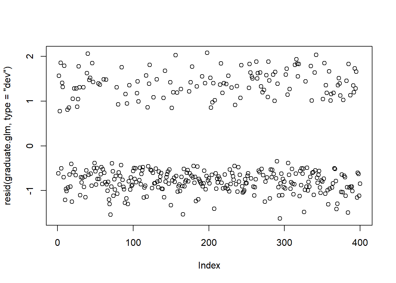
qqnorm(resid(graduate.glm, type="dev"))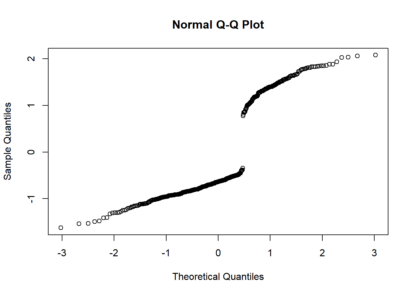
but even these do not help an awful lot. See for example this course for those that are interested.
- Another link function we might consider is the probit link. This is the transformation where the transformed probability is given by \[y^*=\phi^{-1}(p)=\mathbb{\beta} X,\] i.e that the probability of something occuring is based on the normal cumulative density function. In R, we can use the following model
graduate.probit.glm <- glm(admit ~ gre + gpa + rank, data = graduate,
                                          family = binomial (link="probit"))
summary(graduate.probit.glm)
##
## Call:
## glm(formula = admit ~ gre + gpa + rank, family = binomial(link = "probit"),
## data = graduate)
##
## Deviance Residuals:
## Min 1Q Median 3Q Max
## -1.6163 -0.8710 -0.6389 1.1560 2.1035
##
## Coefficients:
## Estimate Std. Error z value Pr(>|z|)
## (Intercept) -2.386836 0.673946 -3.542 0.000398 ***
## gre 0.001376 0.000650 2.116 0.034329 *
## gpa 0.477730 0.197197 2.423 0.015410 *
## rank2 -0.415399 0.194977 -2.131 0.033130 *
## rank3 -0.812138 0.208358 -3.898 9.71e-05 ***
## rank4 -0.935899 0.245272 -3.816 0.000136 ***
## ---
## Signif. codes: 0 '***' 0.001 '**' 0.01 '*' 0.05 '.' 0.1 ' ' 1
##
## (Dispersion parameter for binomial family taken to be 1)
##
## Null deviance: 499.98 on 399 degrees of freedom
## Residual deviance: 458.41 on 394 degrees of freedom
## AIC: 470.41
##
## Number of Fisher Scoring iterations: 4- Repeat the analysis above for the probit link function. Is the model better or worse? Does the predicted admission probability of a student with GRE 700, GPA 3.7, to a rank 2 institution change?
14.1.2 Exercise: Road Bids
- For the ROADBIDS.txt data set, use the above to form a generalised linear model with the logistic link function with response STATUS for regressor variables NUMBIDS and DOTEST.
- By adding terms to the model, for example the cross-term NUMBIDS\(\times\)DOTEST, or quadratic terms, can you find a better model?
14.2 Poisson Regression
Poisson Regression also fits into our GLM framework, although instead of a binary (0/1) response as we had in logistic regression, in Poisson regression the response we measure is some count data: how many times does something occur, for example.
As an example, let x be the temperature on a randomly chosen summer day, and let y be the number of ice creams sold on that day. The data might look like this.
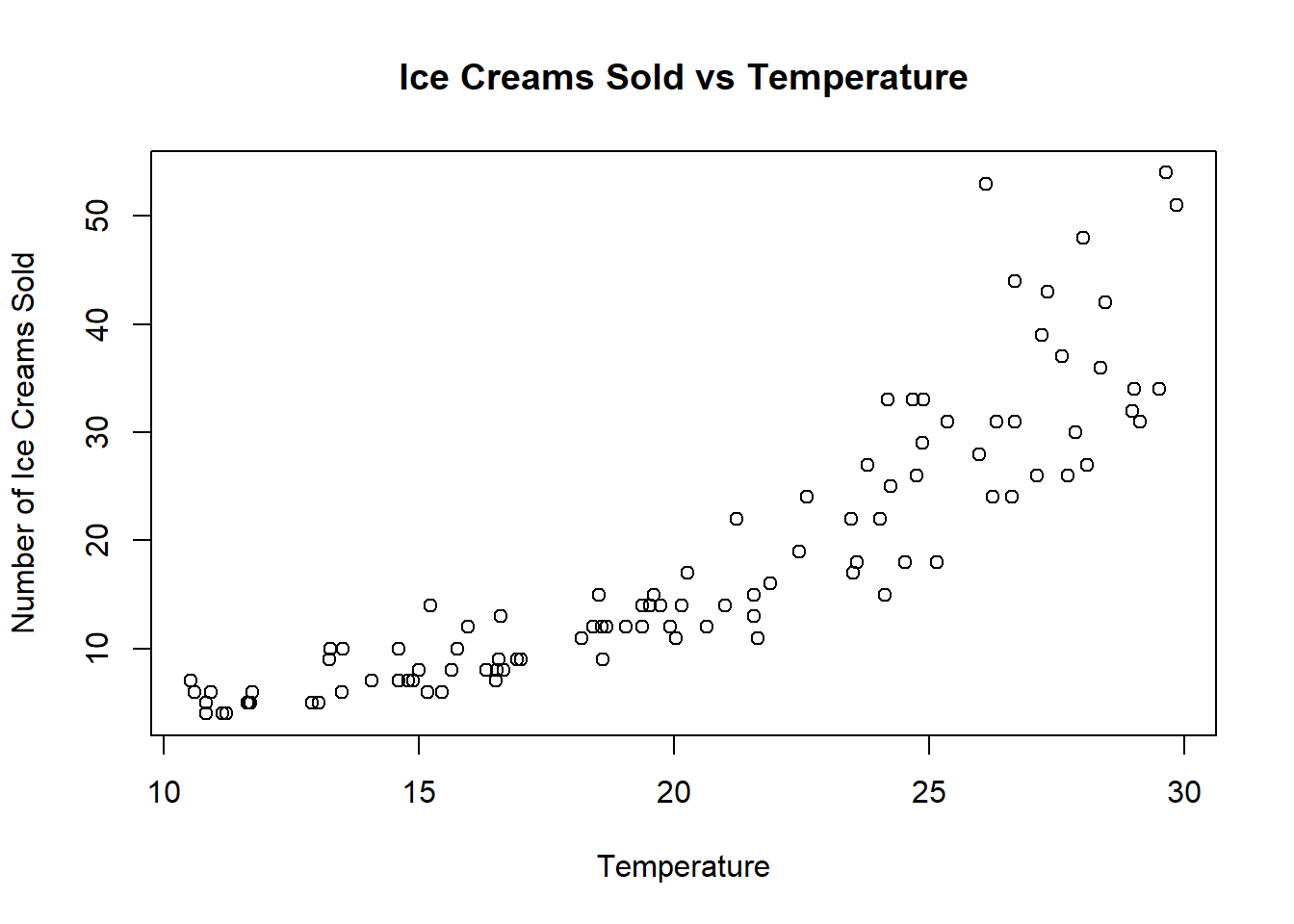
Clearly a linear model does not fit here, but we can find that the following Poisson Regression model is a good fit: \[f(y)=\frac{\mu^y e^{-\mu}}{{y!}}\] where \(log(\mu)=\beta_0+\beta_1x_i\).
14.2.1 Poisson Regression Example
This example inspired by Dataquest
# install.packages("datasets")
library(datasets) # include library datasets after installation
head(warpbreaks)
## breaks wool tension
## 1 26 A L
## 2 30 A L
## 3 54 A L
## 4 25 A L
## 5 70 A L
## 6 52 A LThis data set looks at how many warp breaks occurred for different types of looms per loom, per fixed length of yarn. There are three variables
- breaks (numeric) The number of breaks
- wool (factor) The type of wool (A or B)
- tension (factor) The level of tension, Low, Medium,or High (L, M, H)
There are measurements on 9 looms of each of the six types of warp, for a total of 54 entries in the dataset.
We can view the dependent variable breaks data continuity by creating a histogram:
hist(warpbreaks$breaks)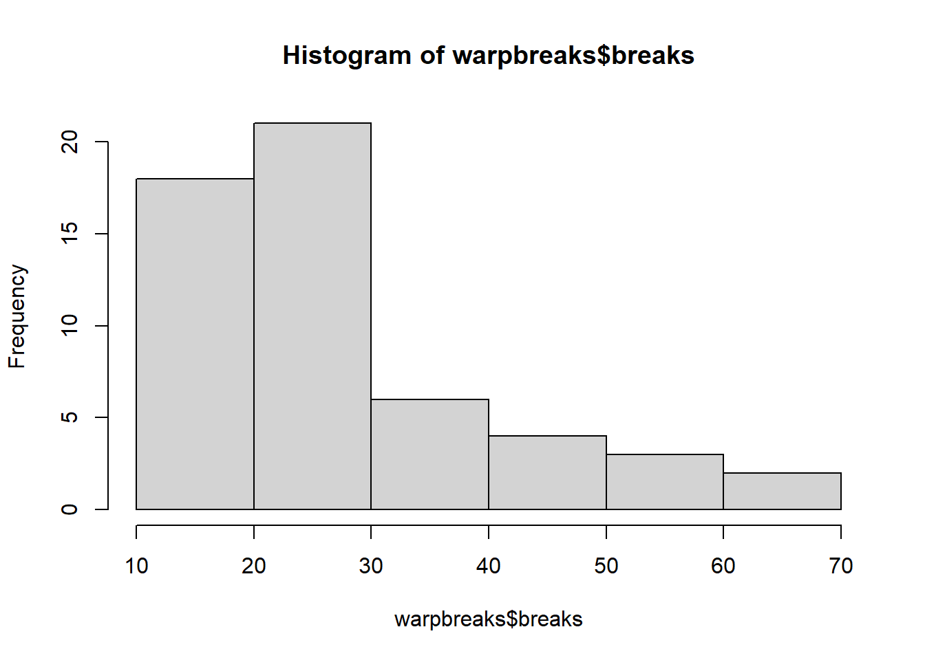
A linear model may well be a bad model:
linear.model <- lm(breaks ~ wool + tension, data=warpbreaks)
summary(linear.model)
##
## Call:
## lm(formula = breaks ~ wool + tension, data = warpbreaks)
##
## Residuals:
## Min 1Q Median 3Q Max
## -19.500 -8.083 -2.139 6.472 30.722
##
## Coefficients:
## Estimate Std. Error t value Pr(>|t|)
## (Intercept) 39.278 3.162 12.423 < 2e-16 ***
## woolB -5.778 3.162 -1.827 0.073614 .
## tensionM -10.000 3.872 -2.582 0.012787 *
## tensionH -14.722 3.872 -3.802 0.000391 ***
## ---
## Signif. codes: 0 '***' 0.001 '**' 0.01 '*' 0.05 '.' 0.1 ' ' 1
##
## Residual standard error: 11.62 on 50 degrees of freedom
## Multiple R-squared: 0.2691, Adjusted R-squared: 0.2253
## F-statistic: 6.138 on 3 and 50 DF, p-value: 0.00123We can plot the residuals, but as in the logistic regression case, the residuals are difficult to interpret, although occasionally any oddities may be clear.
par(mfrow=c(2,2))
plot(linear.model)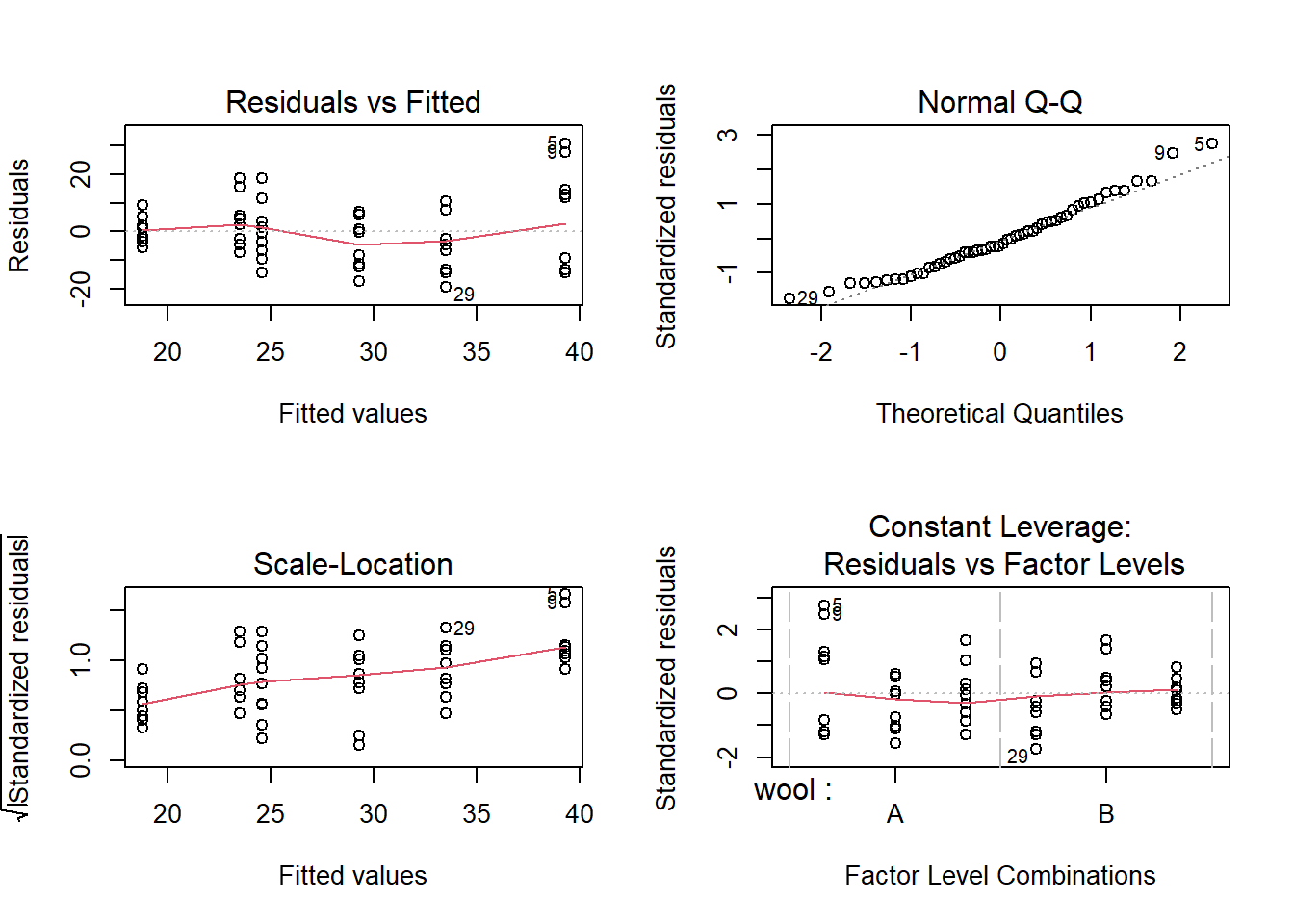
Let’s fit the Poisson model, again using the glm() command.
poisson.model <- glm(breaks ~ wool + tension, data=warpbreaks, family = poisson(link = "log"))
summary(poisson.model)
##
## Call:
## glm(formula = breaks ~ wool + tension, family = poisson(link = "log"),
## data = warpbreaks)
##
## Deviance Residuals:
## Min 1Q Median 3Q Max
## -3.6871 -1.6503 -0.4269 1.1902 4.2616
##
## Coefficients:
## Estimate Std. Error z value Pr(>|z|)
## (Intercept) 3.69196 0.04541 81.302 < 2e-16 ***
## woolB -0.20599 0.05157 -3.994 6.49e-05 ***
## tensionM -0.32132 0.06027 -5.332 9.73e-08 ***
## tensionH -0.51849 0.06396 -8.107 5.21e-16 ***
## ---
## Signif. codes: 0 '***' 0.001 '**' 0.01 '*' 0.05 '.' 0.1 ' ' 1
##
## (Dispersion parameter for poisson family taken to be 1)
##
## Null deviance: 297.37 on 53 degrees of freedom
## Residual deviance: 210.39 on 50 degrees of freedom
## AIC: 493.06
##
## Number of Fisher Scoring iterations: 4To interpret the coefficients, we transform them with the exponential fucntion.
exp(poisson.model$coefficients)## (Intercept) woolB tensionM tensionH
## 40.1235380 0.8138425 0.7251908 0.5954198- R chooses wool A, tension L as the baseline.
- If we move to wool B, the number of breaks is multiplied by 0.81
- If we move to tension M, the number of breaks is multiplied by 0.73
We can also see what out model predicts as a prediction interval for any type of wool and tension.
newdata = expand.grid(wool = c("A","B"), tension = c("L","M","H"))
pl<-predict(linear.model, newdata = newdata, type = "response")
pp<-predict(poisson.model, newdata = newdata, type = "response")
cbind(newdata,pl,pp)
## wool tension pl pp
## 1 A L 39.27778 40.12354
## 2 B L 33.50000 32.65424
## 3 A M 29.27778 29.09722
## 4 B M 23.50000 23.68056
## 5 A H 24.55556 23.89035
## 6 B H 18.77778 19.44298