Chapter 10 Multiple regression
We’ve covered the principles of simple linear regression where we allow one explanatory variable (x) to explain the response variable (y). In this section, we see how to work with more than one explanatory variable in R. The good news is that having understood the principles in the simple linear regression case, much of what we’ve learnt carries through and allows us to use more difficult models with ease.
10.1 Example. Auction Data for Clocks:
In this dataset, we have the price reached in an auction for a number of antique clocks, together with the number of bids made in the auction, and the age of the clocks. Read in the data:
auction<-read.table("https://www.dropbox.com/s/5a8h8h8ynm5zple/GFCLOCKS.txt?dl=1",header=TRUE)
head(auction)
## AGE NUMBIDS PRICE AGE.BID
## 1 127 13 1235 1651
## 2 115 12 1080 1380
## 3 127 7 845 889
## 4 150 9 1522 1350
## 5 156 6 1047 936
## 6 182 11 1979 2002With any dataset I examine, I like to perform some exploratory plots:
library(ggplot2)
ggplot( data=auction, aes(x=AGE, y=PRICE) ) +
    geom_point(  )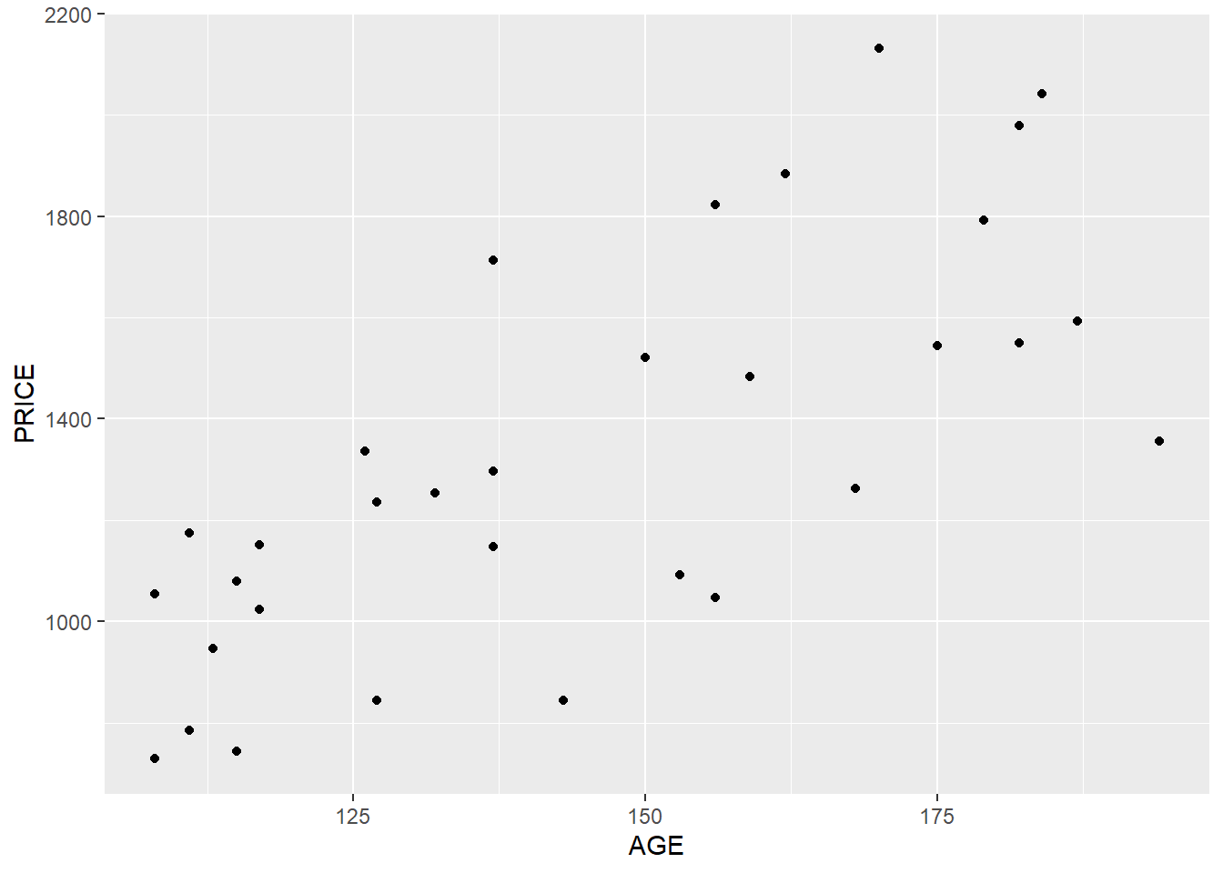
ggplot( data=auction, aes(x=NUMBIDS, y=PRICE) ) +
    geom_point(  )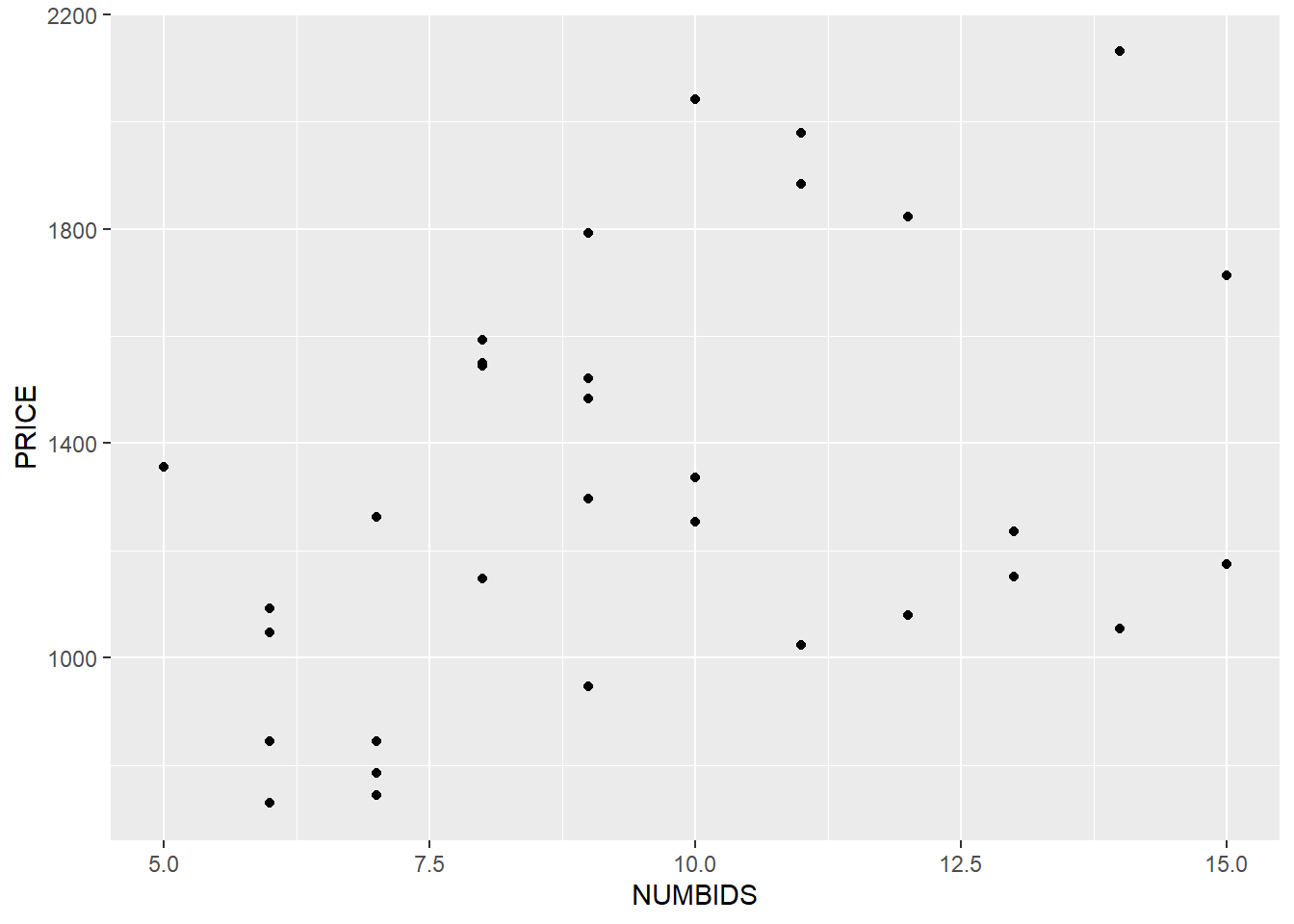
It certainly seems that both AGE and NUMBIDS have a positive correlation with PRICE.
Next I’m going to perform three separate linear models to demonstrate: how does PRICE vary with AGE and NUMBIDS on it’s own.
clocks1.lm<-lm(PRICE~AGE,data=auction)
summary(clocks1.lm)
##
## Call:
## lm(formula = PRICE ~ AGE, data = auction)
##
## Residuals:
## Min 1Q Median 3Q Max
## -485.04 -192.36 31.03 157.50 541.47
##
## Coefficients:
## Estimate Std. Error t value Pr(>|t|)
## (Intercept) -192.047 264.372 -0.726 0.473
## AGE 10.480 1.793 5.844 2.16e-06 ***
## ---
## Signif. codes: 0 '***' 0.001 '**' 0.01 '*' 0.05 '.' 0.1 ' ' 1
##
## Residual standard error: 273.5 on 30 degrees of freedom
## Multiple R-squared: 0.5324, Adjusted R-squared: 0.5168
## F-statistic: 34.15 on 1 and 30 DF, p-value: 2.158e-06clocks2.lm<-lm(PRICE~NUMBIDS,data=auction)
summary(clocks2.lm)##
## Call:
## lm(formula = PRICE ~ NUMBIDS, data = auction)
##
## Residuals:
## Min 1Q Median 3Q Max
## -516.60 -355.05 -29.02 303.23 688.45
##
## Coefficients:
## Estimate Std. Error t value Pr(>|t|)
## (Intercept) 804.91 230.83 3.487 0.00153 **
## NUMBIDS 54.76 23.24 2.356 0.02518 *
## ---
## Signif. codes: 0 '***' 0.001 '**' 0.01 '*' 0.05 '.' 0.1 ' ' 1
##
## Residual standard error: 367.4 on 30 degrees of freedom
## Multiple R-squared: 0.1562, Adjusted R-squared: 0.1281
## F-statistic: 5.553 on 1 and 30 DF, p-value: 0.02518These two models tell us: - AGE is significant in the model when it is the only explanatory variable. - NUMBIDS is significant in the model when it is the only explanatory variable.
Let’s see what happens when we put both AGE and NUMBIDS in the model to try and describe the PRICE.
Formally this is the model \[y_i=\beta_0+\beta_1x_1i+\beta_2x_2i+\epsilon_i\] where - \(y_i\) is the Price of the \(i\)-th clock - \(x_1i\) is the Age of the \(i\)-th clock - \(x_2i\) is the Age of the \(i\)-th clock - \(\beta_0,\beta_1, and \beta_2\) are unknown parameters - \(\epsilon_i\) is the error, with the same assumptions as in the last chapter.
In R we describe this with the model PRICE~NUMBIDS+AGE. This is just R’s way of describing models. We don’t add Numbids and Age together, this just corresponds the additive model we have described just above.
clocks3.lm<-lm(PRICE~NUMBIDS+AGE,data=auction)
summary(clocks3.lm)
##
## Call:
## lm(formula = PRICE ~ NUMBIDS + AGE, data = auction)
##
## Residuals:
## Min 1Q Median 3Q Max
## -206.49 -117.34 16.66 102.55 213.50
##
## Coefficients:
## Estimate Std. Error t value Pr(>|t|)
## (Intercept) -1338.9513 173.8095 -7.704 1.71e-08 ***
## NUMBIDS 85.9530 8.7285 9.847 9.34e-11 ***
## AGE 12.7406 0.9047 14.082 1.69e-14 ***
## ---
## Signif. codes: 0 '***' 0.001 '**' 0.01 '*' 0.05 '.' 0.1 ' ' 1
##
## Residual standard error: 133.5 on 29 degrees of freedom
## Multiple R-squared: 0.8923, Adjusted R-squared: 0.8849
## F-statistic: 120.2 on 2 and 29 DF, p-value: 9.216e-15Both AGE and NUMBIDS are significant in the model in the presence of the other term. Note that the p-value gone down for NUMBIDS when AGE is also fitted, perhaps indicating that the fit is better. From the final plot our final fitted model is that
PRICE= -1338.95 + 85.95 NUMBIDS + 12.74 AGE
i.e. that for each bid in our auction, the price of a clock goes up by $85.95, and for each year of age the price goes up by $12.74. The theoretical starting price of a new clock with no bids would be -$1338.95.
As always, we examine the residuals to check the assumptions of our model.
par(mfrow=c(2,2))
plot(clocks3.lm)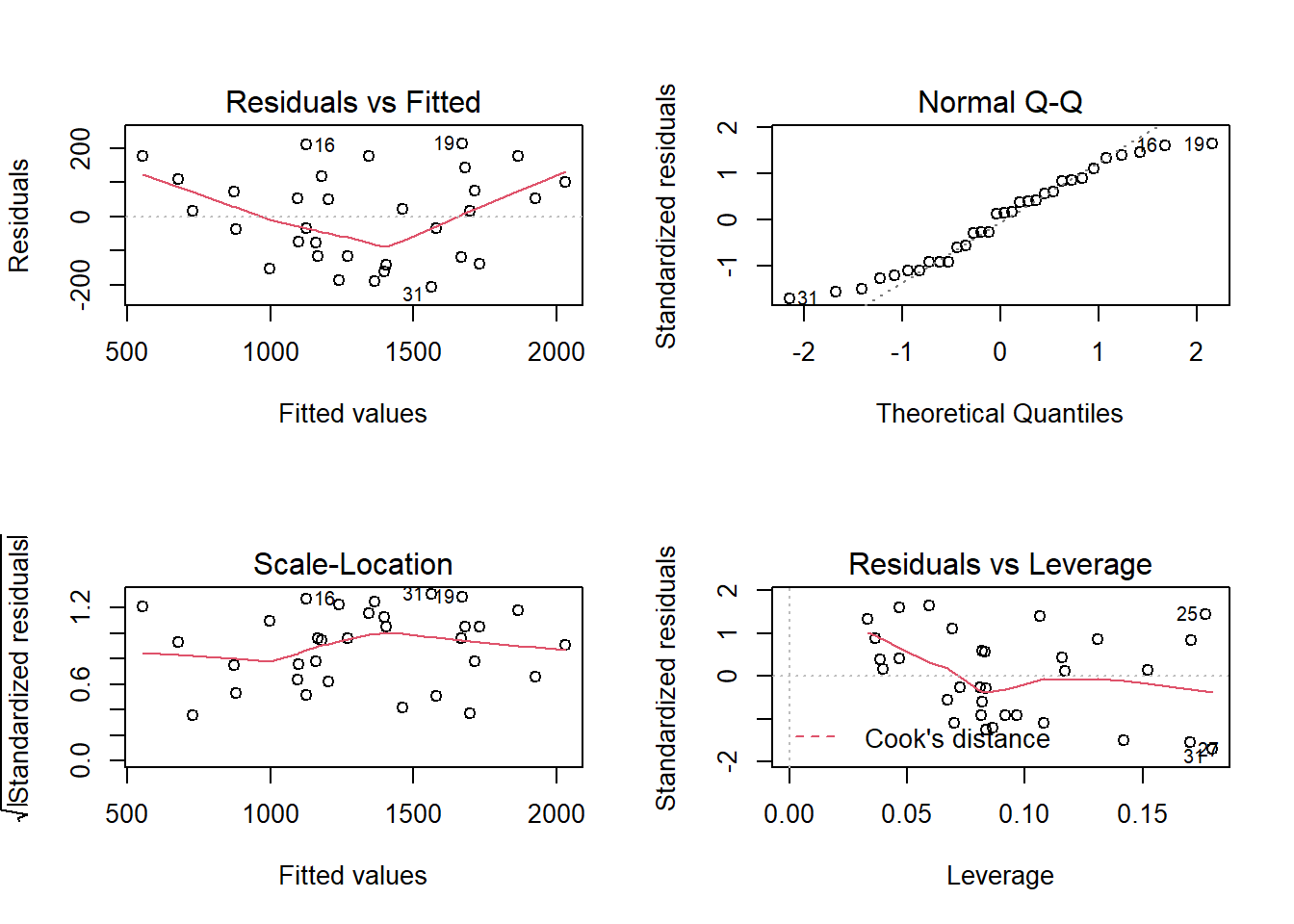
The Q-Q plot perhaps is not ideal, so we are not entirely happy with out model. In practice we might continue with a more sophisticated model.
10.2 Another example: Arsenic
This dataset gives the level of Arsenic for wells in some villages for varying depths of wells, their latitude and longitude, together with some other information we will not use here.
First, lets read the data in, look at the first few rows, and attach the data
arsenic<-read.table("https://www.dropbox.com/s/yxzwgo82ra66ler/ASWELLS.txt?dl=1",header=TRUE,sep="\t")
head(arsenic)
## WELLID UNION VILLAGE LATITUDE LONGITUDE DEPTH.FT YEAR KIT.COLOR ARSENIC
## 1 10 Araihazar Krishnapura 23.7887 90.6522 60 1992 Red 331
## 2 14 Araihazar Krishnapura 23.7886 90.6523 45 1998 Red 302
## 3 30 Araihazar Krishnapura 23.7880 90.6517 45 1995 Red 193
## 4 59 Araihazar Krishnapura 23.7893 90.6525 125 1973 Red 232
## 5 85 Duptara Hatkholapara 23.7920 90.6140 150 1997 Green 19
## 6 196 Brahmandi Narindi 23.7817 90.6250 60 1993 Green 33We have one bit of housekeeping to do first. If we look at the 199th Depth reading, it is denoted as * in the original data. We need to tell R that “*” means this data is missing, and set this value to NA (which is how R denotes missing data). Because we initially had a non-numeric value, we tell R that this is a numeric variable here.
arsenic$DEPTH.FT[199]## [1] "*"arsenic$DEPTH.FT[199]<-NA
arsenic$DEPTH.FT<-as.numeric(arsenic$DEPTH.FT)Now we perform some initial data analysis with some exploratory plots. The pairs command is useful to see many relationships at once between pairs of variables.
pairs(~LATITUDE +LONGITUDE +DEPTH.FT+ARSENIC,data=arsenic)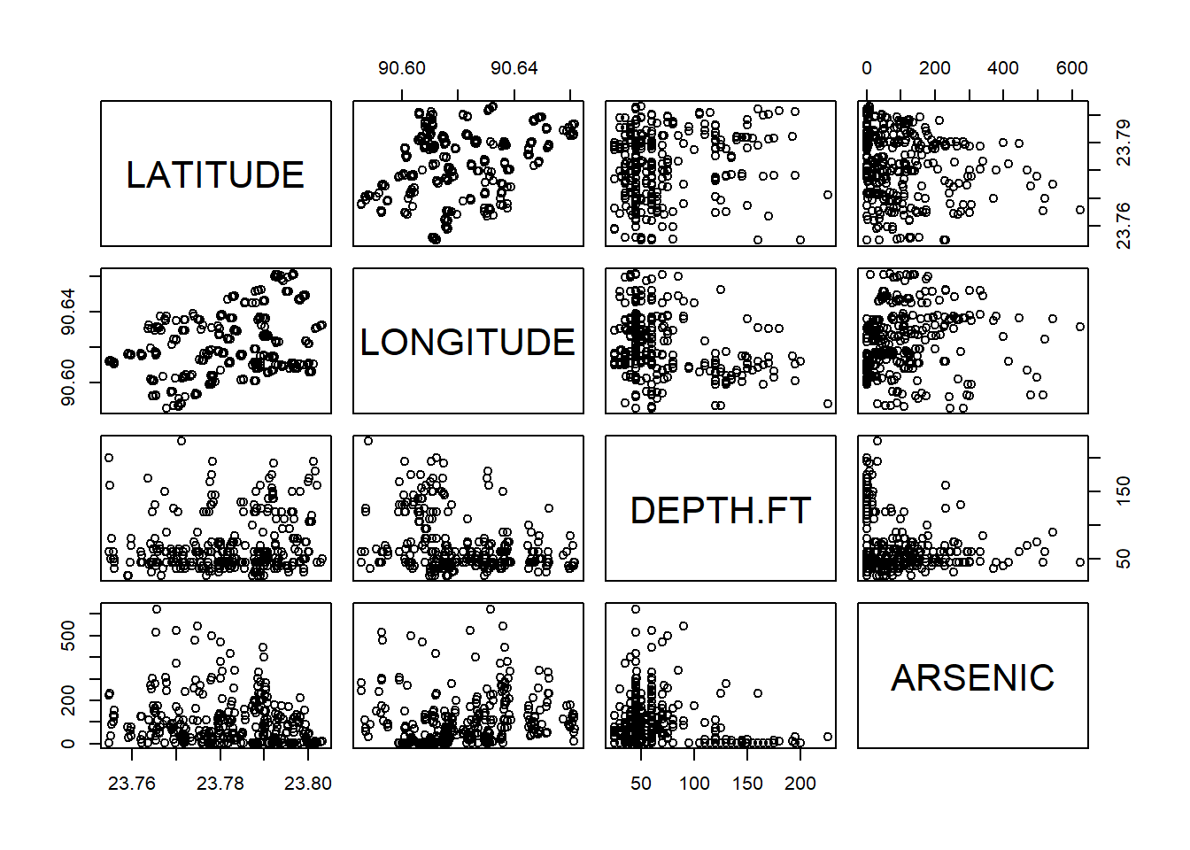
It is more challenging here to see any relationship for sure.
Let’s put all our terms in a linear model.
arsenic.lm<-lm(ARSENIC~LONGITUDE+LATITUDE+DEPTH.FT,data=arsenic)
summary(arsenic.lm)
##
## Call:
## lm(formula = ARSENIC ~ LONGITUDE + LATITUDE + DEPTH.FT, data = arsenic)
##
## Residuals:
## Min 1Q Median 3Q Max
## -134.43 -65.50 -26.82 27.03 469.17
##
## Coefficients:
## Estimate Std. Error t value Pr(>|t|)
## (Intercept) -8.699e+04 3.122e+04 -2.787 0.00564 **
## LONGITUDE 1.544e+03 3.730e+02 4.139 4.46e-05 ***
## LATITUDE -2.220e+03 5.268e+02 -4.215 3.25e-05 ***
## DEPTH.FT -3.493e-01 1.566e-01 -2.230 0.02643 *
## ---
## Signif. codes: 0 '***' 0.001 '**' 0.01 '*' 0.05 '.' 0.1 ' ' 1
##
## Residual standard error: 103.3 on 323 degrees of freedom
## (1 observation deleted due to missingness)
## Multiple R-squared: 0.1281, Adjusted R-squared: 0.12
## F-statistic: 15.81 on 3 and 323 DF, p-value: 1.282e-09All the terms are needed in our model; the last column for our coefficients shows small values for all our slope coefficients, so it shows that we can reject the hypothesis that any of them is zero. Moreover, the F statistic and associated p-value at the bottom show that the regression as a whole is significant, which is expected as all our coefficients are highly sufficient. We check the assumptions of the model by checking the residuals:
plot(arsenic.lm)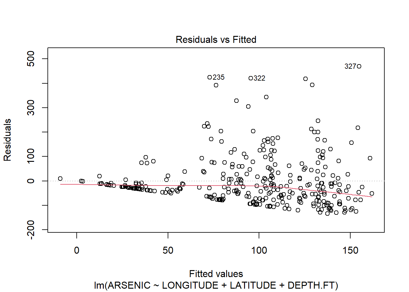
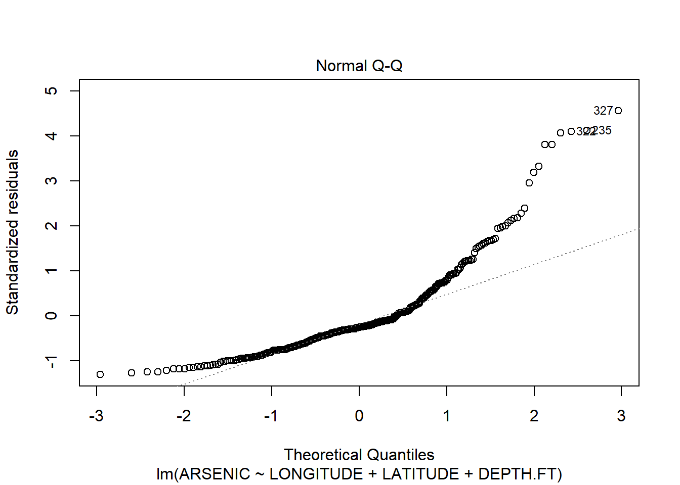
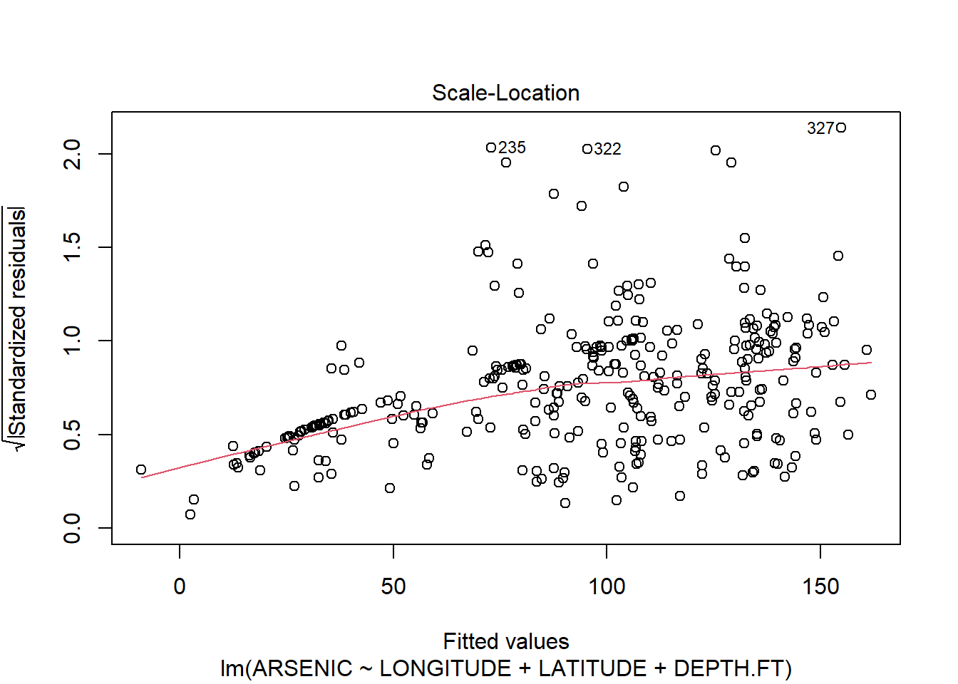
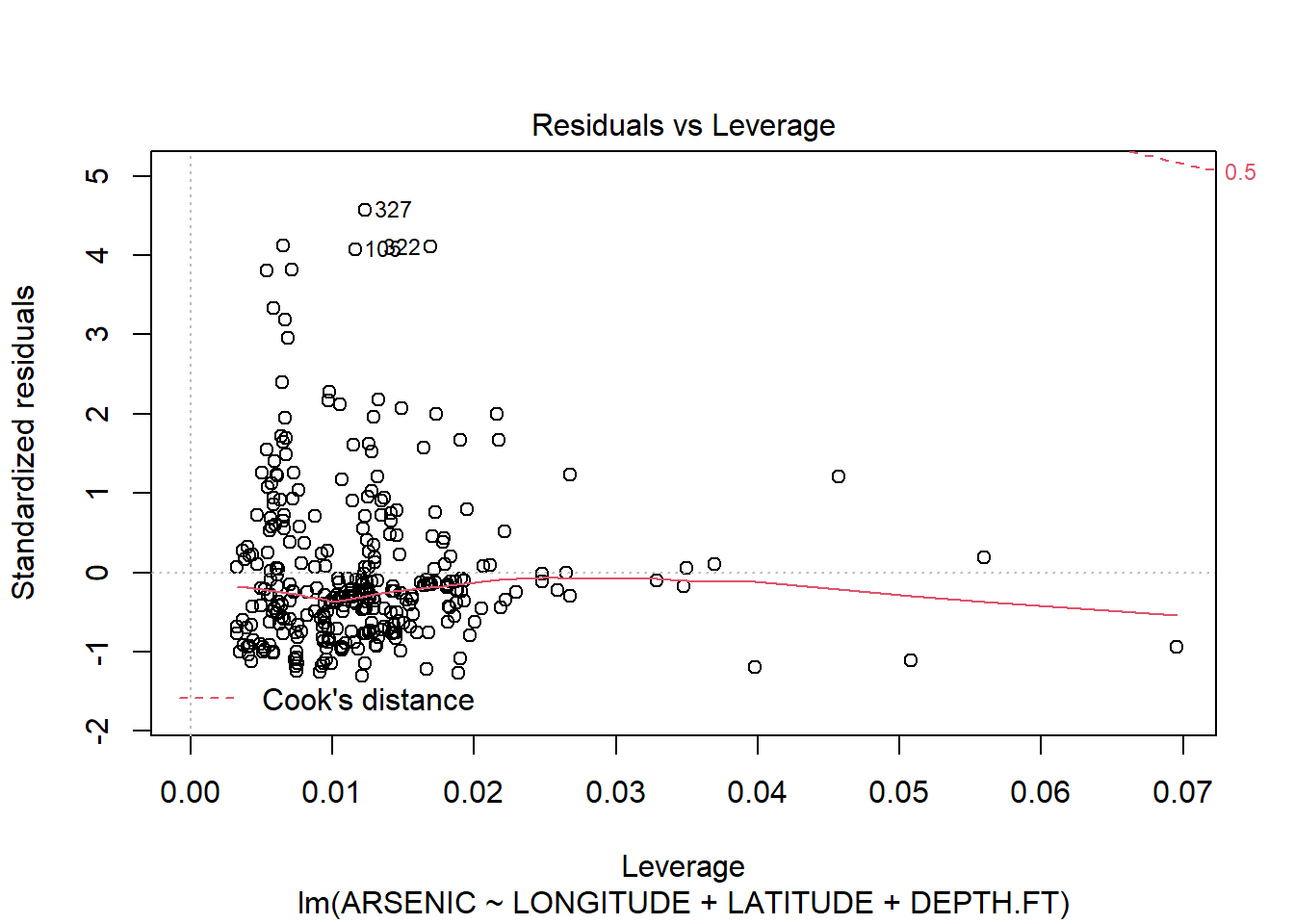
The residuals clearly show us that the model does not fit! The Resuduals vs fitted plot shows a classic funnel shape, implying that the variance increases as the fitted value increases. We can also see this on the original scatter plots. The Q-Q plots also suggest non-normality.
We see later in the course that one way to deal with this heteroskedasticity (differing variances) is to transform y to log(y). In this case we can do this easily.
arsenic.lm2<-lm(log(ARSENIC)~LONGITUDE+LATITUDE+DEPTH.FT,data=arsenic)
summary(arsenic.lm2)
##
## Call:
## lm(formula = log(ARSENIC) ~ LONGITUDE + LATITUDE + DEPTH.FT,
## data = arsenic)
##
## Residuals:
## Min 1Q Median 3Q Max
## -4.1124 -1.1567 0.1471 1.1436 3.4359
##
## Coefficients:
## Estimate Std. Error t value Pr(>|t|)
## (Intercept) -2.611e+03 4.806e+02 -5.432 1.10e-07 ***
## LONGITUDE 4.332e+01 5.743e+00 7.543 4.71e-13 ***
## LATITUDE -5.511e+01 8.110e+00 -6.795 5.24e-11 ***
## DEPTH.FT -1.338e-02 2.411e-03 -5.551 5.94e-08 ***
## ---
## Signif. codes: 0 '***' 0.001 '**' 0.01 '*' 0.05 '.' 0.1 ' ' 1
##
## Residual standard error: 1.59 on 323 degrees of freedom
## (1 observation deleted due to missingness)
## Multiple R-squared: 0.3533, Adjusted R-squared: 0.3473
## F-statistic: 58.81 on 3 and 323 DF, p-value: < 2.2e-16plot(arsenic.lm2)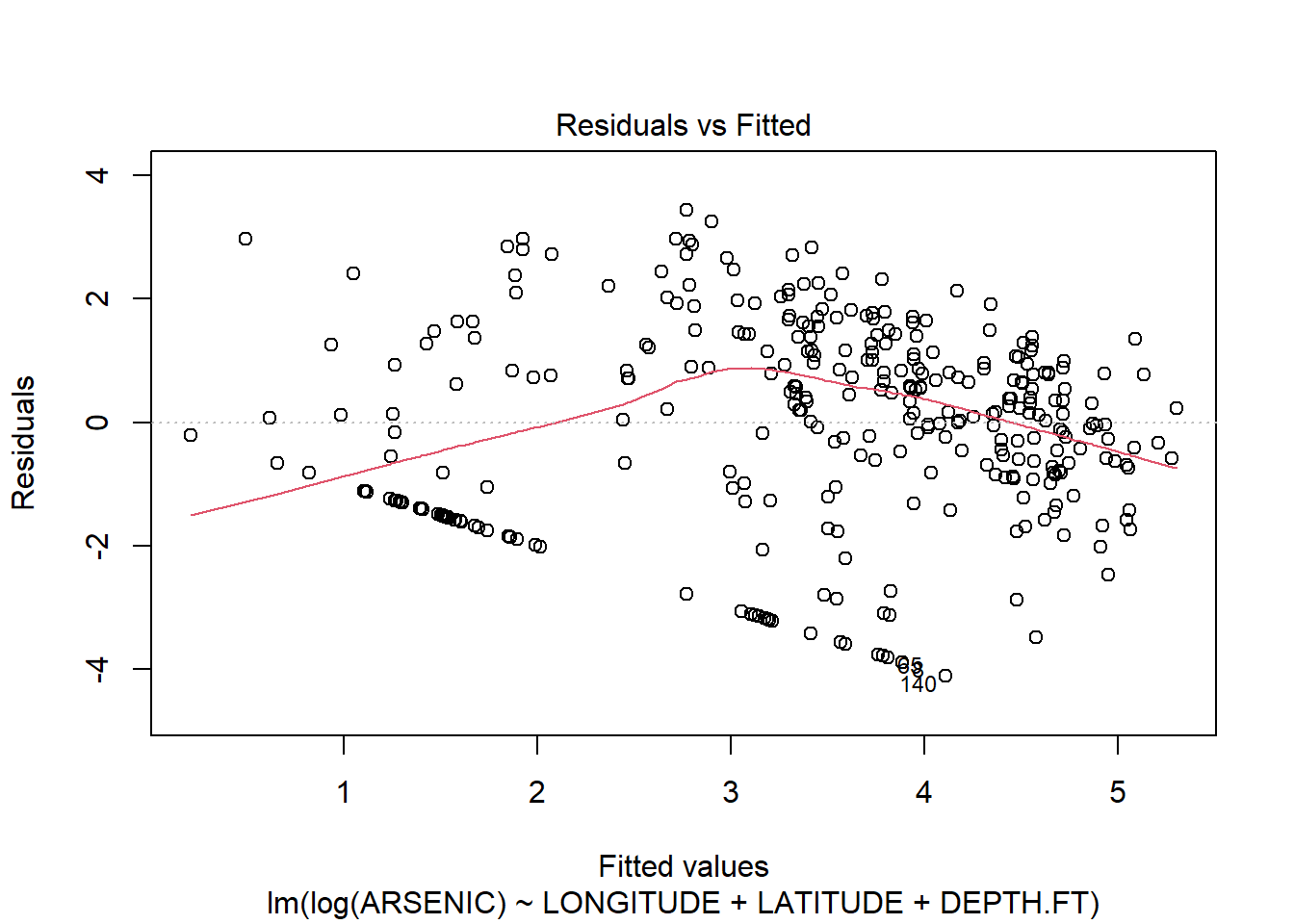
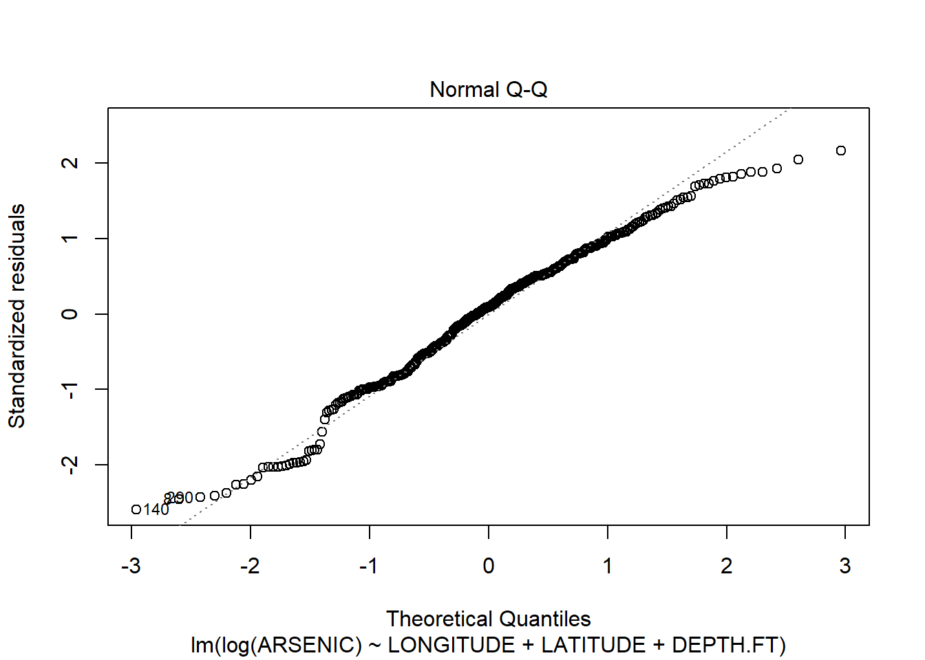
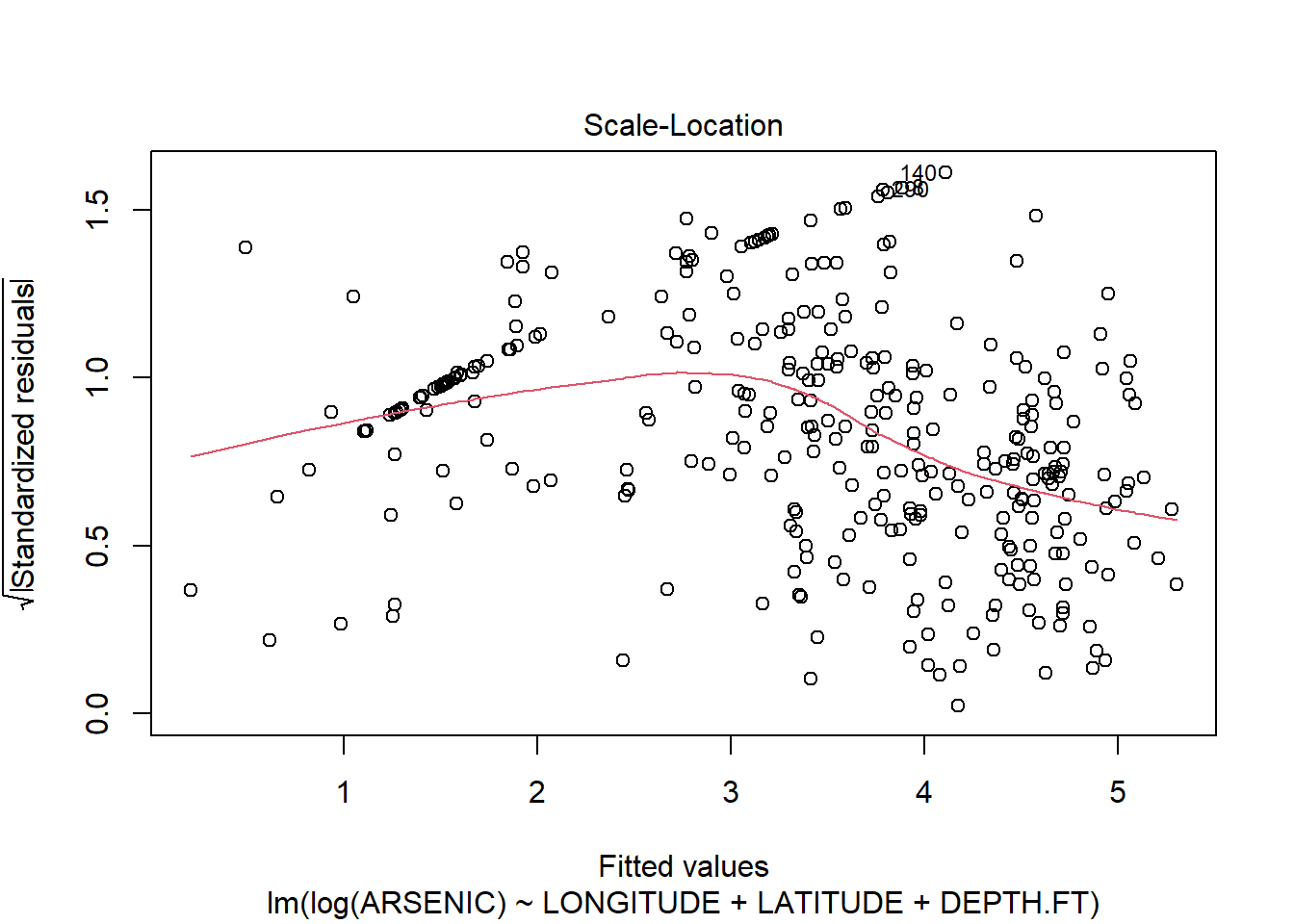
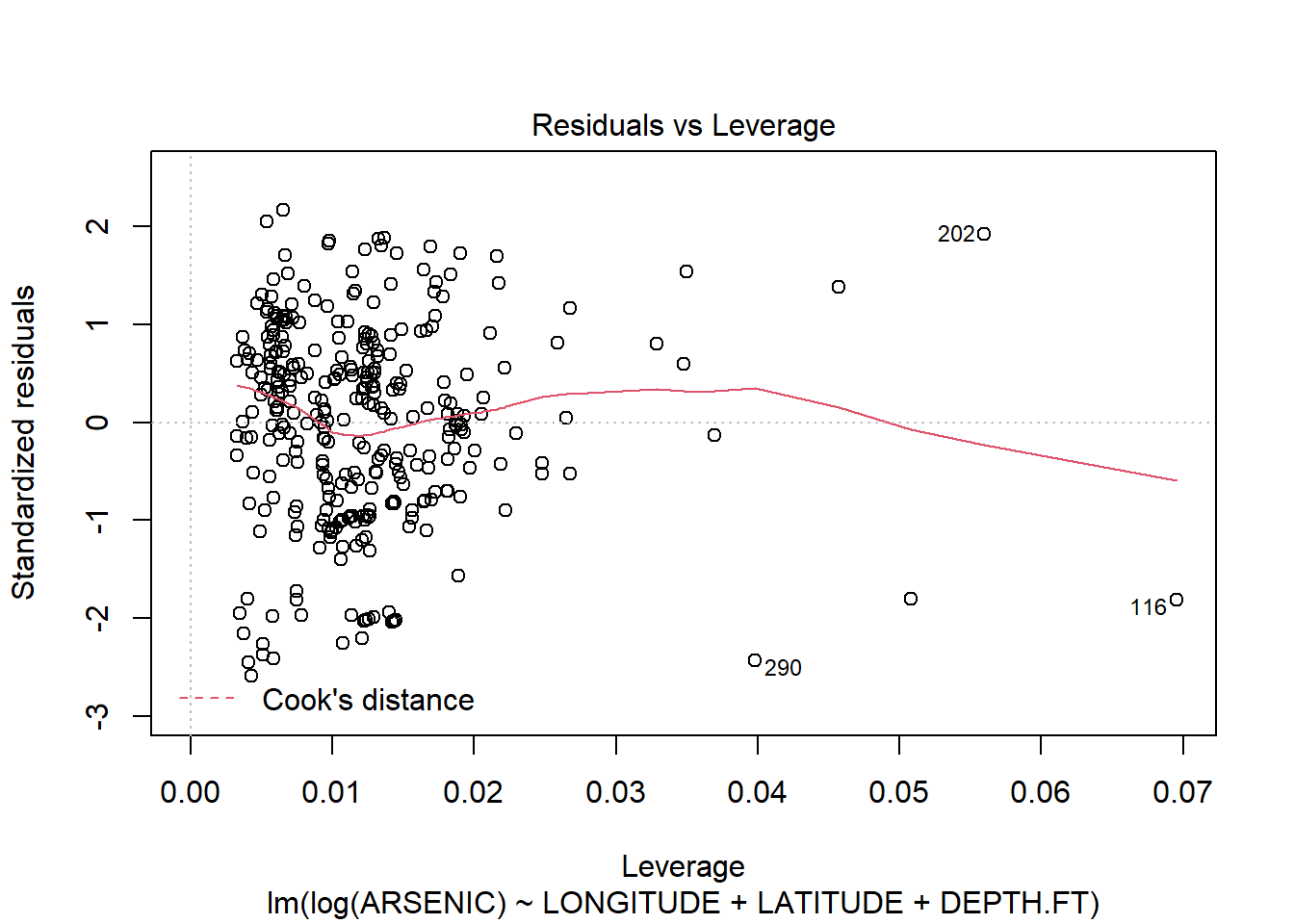
There are still some problems, but the fit of the model is much improved.(Note a linear model is probably not the right model for this type of data: we will see later in the course when we look at the general linear model how we might deal with this “Count” data. )
10.3 Polynomial regression example. Sidewalls from aeroplanes.
In this example we see how the cost of Airplane Sidewalls varies with Lot Size.
Read the data in and plot the data.
x<-c(20,25,30,35,40,50,60,65,70,75,80,90)
y<-c(1.81,1.7,1.65,1.55,1.48,1.4,1.3,
1.26,1.24,1.21,1.2,1.18)
plot(x,y,main="Cost of Airplane sidepanels",
ylab="Average cost per unit (x100$)",xlab="Lot size")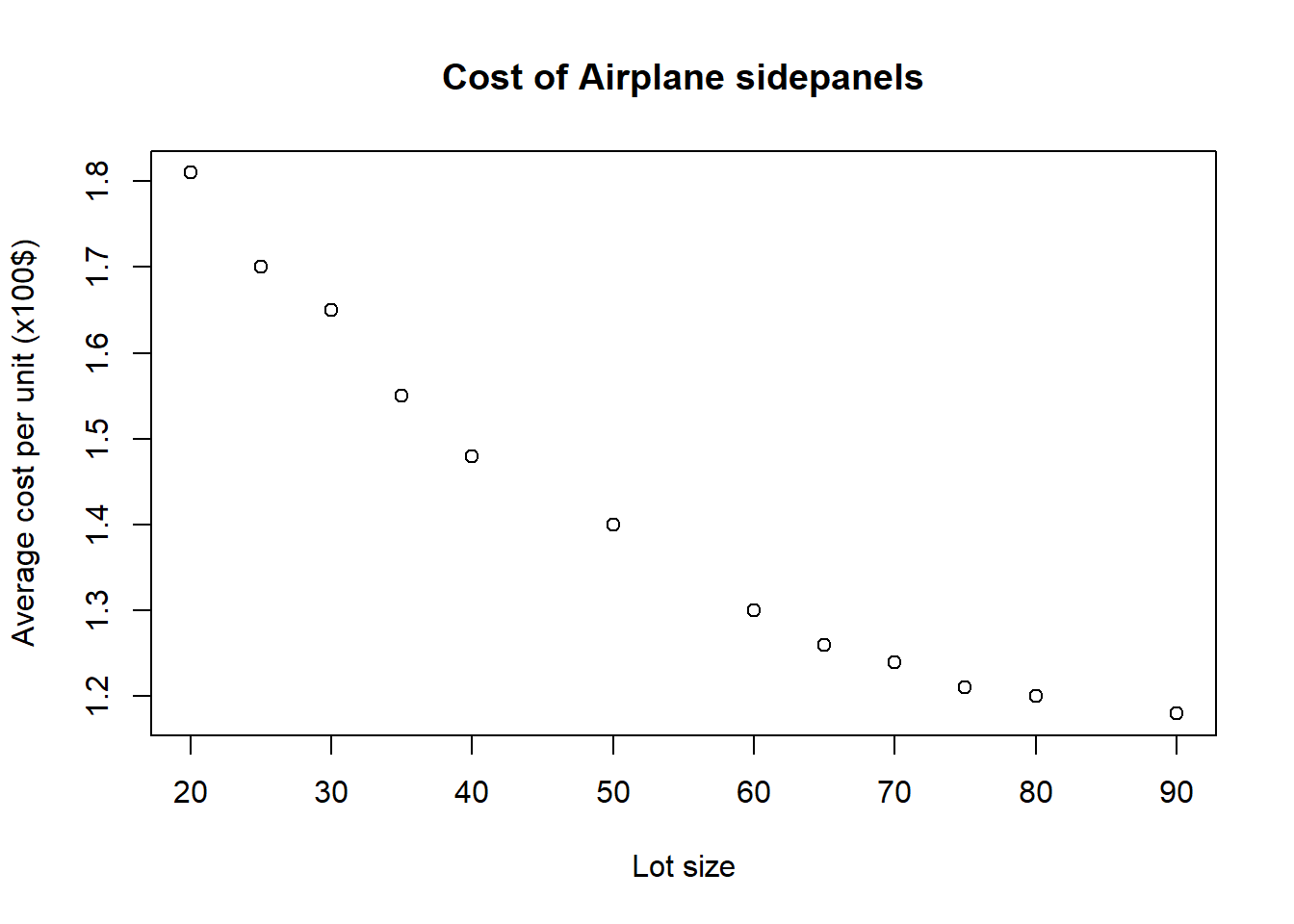 Form a linear model and plot the line of best fit in the normal way.
sidepanels.lm<-lm(y~x)
plot(x,y,main="Cost of Airplane sidepanels",
       ylab="Average cost per unit (x100$)",xlab="Lot size")
abline(sidepanels.lm)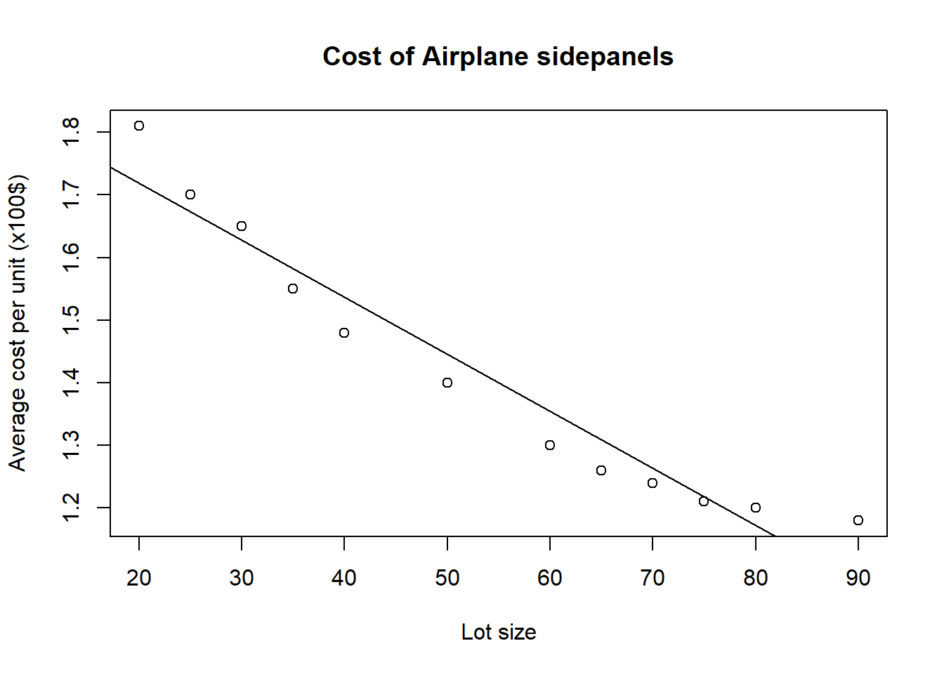
Examine the model and plot the residuals.
summary(sidepanels.lm)##
## Call:
## lm(formula = y ~ x)
##
## Residuals:
## Min 1Q Median 3Q Max
## -0.05634 -0.04621 -0.01557 0.02728 0.09869
##
## Coefficients:
## Estimate Std. Error t value Pr(>|t|)
## (Intercept) 1.9003631 0.0425582 44.65 7.63e-13 ***
## x -0.0091006 0.0007362 -12.36 2.21e-07 ***
## ---
## Signif. codes: 0 '***' 0.001 '**' 0.01 '*' 0.05 '.' 0.1 ' ' 1
##
## Residual standard error: 0.05687 on 10 degrees of freedom
## Multiple R-squared: 0.9386, Adjusted R-squared: 0.9324
## F-statistic: 152.8 on 1 and 10 DF, p-value: 2.209e-07par(mfrow=c(2,2))
plot(sidepanels.lm)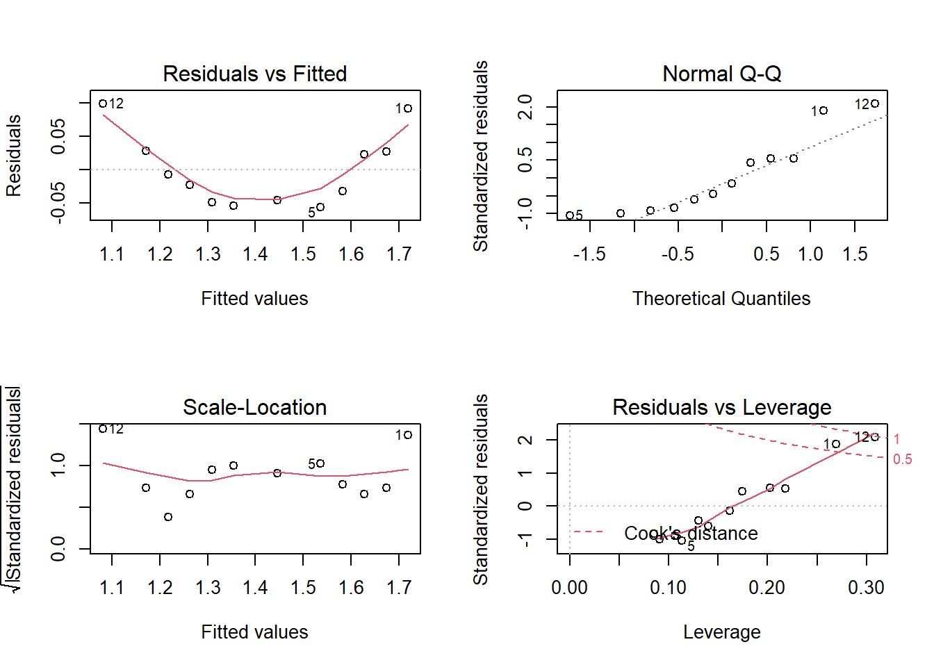
Clearly the linear model does not fit. Let us examine polynomial models. For example these might be models of the form
\[y_i=\beta_0+\beta_1x_i+\beta_2x_i^2+\epsilon_i\]
\[y_i=\beta_0+\beta_1x_i+\beta_2x_i^2+\beta_3x_i^3+\epsilon_i\]
We introduce new variables xSquare and xCube (representing \(x^2\) and \(x^3\), of course, and form models with these terms included.)
# Form x^2, x^3
xSquare<-x*x
xCube<-x*x*x

# Plot the polynomial quadratic and cubic linear models
sidepanels.lm2<-lm(y~x+xSquare)
summary(sidepanels.lm2)
##
## Call:
## lm(formula = y ~ x + xSquare)
##
## Residuals:
## Min 1Q Median 3Q Max
## -0.0174763 -0.0065087 0.0001297 0.0071482 0.0151887
##
## Coefficients:
## Estimate Std. Error t value Pr(>|t|)
## (Intercept) 2.198e+00 2.255e-02 97.48 6.38e-15 ***
## x -2.252e-02 9.424e-04 -23.90 1.88e-09 ***
## xSquare 1.251e-04 8.658e-06 14.45 1.56e-07 ***
## ---
## Signif. codes: 0 '***' 0.001 '**' 0.01 '*' 0.05 '.' 0.1 ' ' 1
##
## Residual standard error: 0.01219 on 9 degrees of freedom
## Multiple R-squared: 0.9975, Adjusted R-squared: 0.9969
## F-statistic: 1767 on 2 and 9 DF, p-value: 2.096e-12sidepanels.lm3<-lm(y~x+xSquare+xCube)
summary(sidepanels.lm3)##
## Call:
## lm(formula = y ~ x + xSquare + xCube)
##
## Residuals:
## Min 1Q Median 3Q Max
## -0.014055 -0.006793 0.001309 0.002919 0.017575
##
## Coefficients:
## Estimate Std. Error t value Pr(>|t|)
## (Intercept) 2.253e+00 5.612e-02 40.143 1.63e-10 ***
## x -2.625e-02 3.639e-03 -7.213 9.13e-05 ***
## xSquare 1.991e-04 7.042e-05 2.828 0.0222 *
## xCube -4.459e-07 4.208e-07 -1.059 0.3203
## ---
## Signif. codes: 0 '***' 0.001 '**' 0.01 '*' 0.05 '.' 0.1 ' ' 1
##
## Residual standard error: 0.01211 on 8 degrees of freedom
## Multiple R-squared: 0.9978, Adjusted R-squared: 0.9969
## F-statistic: 1195 on 3 and 8 DF, p-value: 6.049e-11Our conclusions from sidepanel example:
- The simple linear model, \(Y=\beta_0+\beta_1x+\epsilon_i\) does not appear to fit the data very well. The residual plots show clear evidence of non-linearity (the top-left plot is curved), and also the top-right Q-Q plot shows signs that the residuals are not normally distributed. A visual inspection of the scatterplot of y against x suggests a quadratic model might be more appropriate.
- The quadratic model, \(Y=\beta_0+\beta_1x+\beta_{2}x^2+\epsilon_i\) seems to fit better. The value of \(R^2\) (0.9975) is higher than for the linear model (0.9386), as is the adjusted \(R^2\) (0.9969 vs. 0.9324). The value of \(R^2\) for the quadratic model is close to 1, the theoretical maximum, and here 99.75% of the variation in the data is explained by the model.
- In this quadratic model, the two hypothesis tests for the values of \(\beta_1\) and \(\beta_2\) show that there is very strong evidence to conclude that they are both non-zero (the values of the T statistic are very high, meaning that the p-values are tiny). Thus, we conclude that there is strong evidence that both a linear and a quadratic term (\(x\) and \(x^2\)) are needed in the model.
- We do not choose a cubic model as adding an extra \(x^3\) term only increases the already high value of \(R^2\) by a very small amount compared to the quadratic model, and the adjusted \(R^2\) statistic does not increase. Moreover, by adding a cubic term, we see from a t-test that it is not needed in the model in the presence of the other terms. By the principle of parsimony, we accept the simpler model, and conclude that our quadratic model \(Y=\beta_0+\beta_1x+\beta_{2}x^2+\epsilon_i\) fits the data best of those we have studied.
We plot the final scatterplot, model, and check the residuals.
plot(x,y,main="Cost of Airplane sidepanels",ylab="Average cost per unit (x100$)",xlab="Lot size")
lines(x, predict(sidepanels.lm2), col="red")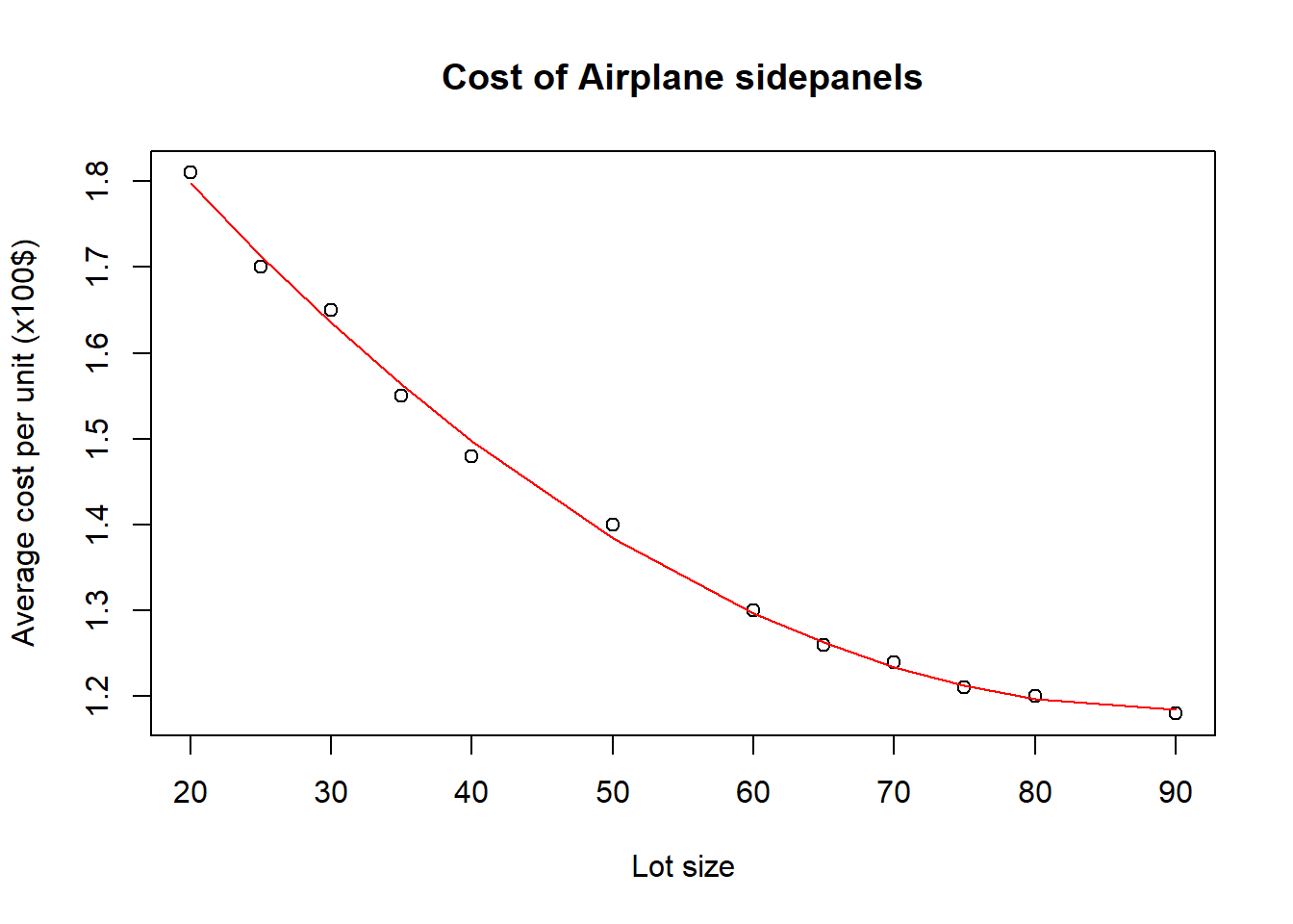
par(mfrow=c(2,2))
plot(sidepanels.lm2)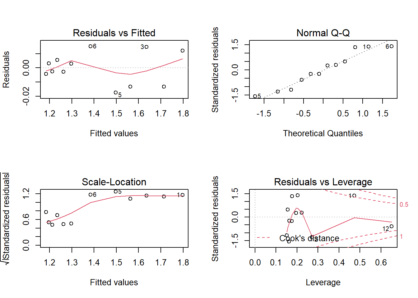
The residual plots for the quadratic model also show no reason to doubt the model assumptions; the residual plot (top-left) shows an equal number of points above and below the line, for example, and the distribution of residuals appears fairly random. The Q-Q plot also shows little reason to doubt the model, as all the points are close to the line.
10.4 Exercises
10.4.1 Exercise 1: Reviewing Simple Linear Regression, plus polynomial regression
Janka hardness is an important structural property of Australian timbers which is difficult to measure directly. However, it is related to the density of the timber which is comparatively easy to measure. Therefore it is desirable to fit a model enabling the Janka hardness to be predicted from the density. The Janka hardness and density of 36 Australian eucalypt hardwoods are available.
library(readr)
janka <- read_table2("https://www.dropbox.com/s/uuurt51woofo9q9/janka.txt?dl=1")
## Warning: `read_table2()` was deprecated in readr 2.0.0.
## Please use `read_table()` instead.##
## -- Column specification ---------------------------------------------------------------------
## cols(
## Density = col_double(),
## Hardness = col_double()
## )head(janka)## # A tibble: 6 x 2
## Density Hardness
## <dbl> <dbl>
## 1 24.7 484
## 2 24.8 427
## 3 27.3 413
## 4 28.4 517
## 5 28.4 549
## 6 29 648Hardness is considered the dependent (\(y\)) variable and Density the independent (\(x\))
variable.
- Plot
HardnessagainstDensity. Is there a relationship between these two variables? Is it clear that it is linear? - Fit the least squares regression line, selecting hardness as the response and density as the predictor.
- Now look at the residual plots. First, look at residuals versus fitted values. A random scatter here suggests that the assumption of equal variances is OK. A funnel shape suggests the variance is increasing with the mean. Is that what you see here?
- Next look at the normal plot. Is there a possible problem?
- The fact that the normality assumption is suspect and that the
variance may be increasing suggests we should transform the dependent
variable hardness. Define a new variable
logHby typinglogH<-log(Hardness)to set the new variable as the (natural) logarithm of \(Y\). - Now fit a simple linear regression model
to
logH. Look at the normal plot and the plot of residuals versus fitted values. The normal plot is now OK but the plot of residuals versus fitted values shows a distinct pattern. Small and large values of fitted values have mainly negative residuals and moderate values positive residuals. This suggests that a quadratic term in density should be included in the model. - Fit the quadratic regression model \[ \log y_i = \beta_0 + \beta_1 x_i + \beta_2 x_i^2 + \varepsilon_i .\] Note the regression equation. Look at the T values next to the coefficients and the associated p-values. The p-values are all small, suggesting that the coefficients are significantly different from zero and that all the terms should be included in the model.
- Check the residual plots and see if they cast any doubt on the model.
- Try adding a cubic term to the model. Is there any evidence that this term is needed?
- You could also try a different transformation of the y term. A square root or reciprocal are possibilities.
10.4.2 Exercise 2: Car Sales
Data on a particular year’s sales (y in $100,000) in 15 sales districts are given in the file sales.txt available on the course dropbox. A company is interested in the dependence of sales on promotional expenditure (\(x_1\) in $1000), the number of active accounts (\(x_2\)), the district potential (\(x_3\) coded), and the number of competing brands (\(x_4\)).
Perform simple linear regression analysis of sales \(y\) for each explanatory variable separately, that is do analyses of dependence of \(y\) on each of the \(x_i\), \(i=1,2,3,4\). Do a separate
lmcommand for each potential model, and for each model:- Test the significance of the regression.
- Comment on the residual plots.
- Note also the value of the coefficient of determination (\(R^2\)) displayed in the of a linear model object. As discussed in lectures this value tells you the percentage of variation explained by the model; we want this value to be high (as close to 100% as possible). Comparing \(R^2\) for two different models is one way of helping us to select which model is better.
Fit a multiple linear regression model \[y_i=\beta_0+\beta_1x_{1i}+\beta_2x_{2i}+\epsilon_i\] and comment on the values of \(S\), \(R^2\) and the residual plots. (You can do this in R by typing ).
Add \(x_3\) to the previous model (of point 2) and comment on the value of \(R^2\) and the residual plots.
Further, add \(x_4\) to the model and comment on the value of \(R^2\) and the residual plots.
For this last model with all the regressors included:
- Test the significance of the regression.
- Test the significance of each of the regression parameters \(\beta_j\), \(j=0,1,2,3,4\).
- One of the parameters is non-significant. Remove the respective variable and reanalyze the data with all other variables in the model.
- Comment on the residual plots for this reduced model.
Try taking out from this model the variable which fitted least well on its own and comment.
10.4.3 Exercise 3: Chemical Reactions
An experiment was carried out on a biochemical process which involves converting a solid substrate into a liquid using an enzyme reaction at high temperatures. The objective of this experiment was to see whether the enzyme activity is affected by the total solids content and the outlet temperature. The datafile chemical.txt contains three columns corresponding to the total solids content \(x_1\), the outlet temperature \(x_2\) and the enzyme activity \(y\). (Note this file does not have a header, so you should add your own labels.)
- Fit a multiple regression model for \(y\) against regressor variables \(x_1\) and \(x_2\).
- Now fit a second-order polynomial regression model. To do this,
create new objects corresponding to \(x_1^2,x_2^2,x_1x_2\), e.g. by doing, for example
x_1_sq<-x_1^2and then fit the second order model (the model containing all the terms \(x_1,x_2, x_1^2,x_2^2,x_1x_2\)). - This is something not covered in lectures- and those with more of a statistical background might find it interesting
- What is the difference in the residual sums of squares for the new model compared to the old model?. This is \(SS_{\mbox{extra}}\) for adding the three second-order terms into the model. To determine whether the change in sum of squares is significant, we must test the hypothesis \[H_0 : \beta_q = \beta_{q+1} = \ldots = \beta_{p-1} =0\] versus \[H_1 \; : \; \mbox{at least one of these is non-zero.}\] It can be shown that, if \(H_0\) is true, \[F = \frac{SS_{\mbox{extra}}/(p-q)}{s^2} \sim F^{p-q}_{n-p} \] So we reject \(H_0\) at the \(\alpha\) level if \(F > F^{p-q}_{n-p}(\alpha)\) and conclude there is sufficient evidence to show some (but not necessarily all) of the `extra’ variables \(x_{q}, \ldots, x_{p-1}\) should be included in the model.
- Use this \(SS_{\mbox{extra}}\) and the test described above to test whether the second order model is better than the first order model, i.e. in the model \[E(Y_i) = \beta_0 + \beta_1x_{1i} + \beta_2x_{2i} + \beta_{11}x_{1i}^2 + \beta_{22}x_{2i}^2 + \beta_{12}x_{1i}x_{2i}\], suppose \(H_0: \beta_{11} = \beta_{22} = \beta_{12} = 0\). What is your alternative hypothesis?
- What do you conclude from the test?
- As usual, R gives hypothesis tests for each parameter. What are the null and alternative hypotheses here? What can you conclude from these?
- Refit the model without the variable whose coefficient is insignificant. Check the residuals.
- What is the value of \(R^2\) for the final model? Is this substantially different from the full second-order polynomial model?
- How can you interpret the final model you have fitted in non-technical language?
- There are some points which look like they are clearly not correct; perhaps they have been recorded incorrectly, or something went wrong with the experiment. We call these outliers. Can you see which these are? If you have time left, you may want to re-analyze the data, but with these outliers deleted. Do you get a better model?