OR-Notes are a series of introductory notes on topics that fall under the broad heading of the field of operations research (OR). They were originally used by me in an introductory OR course I give at Imperial College. They are now available for use by any students and teachers interested in OR subject to the following conditions.
A full list of the topics available in OR-Notes can be found here.
To get some insight into solving LP's consider the Two Mines problem that we had before - the LP formulation of the problem was:
minimise
      180x + 160y
subject to
      6x + y >= 12
      3x + y >= 8
      4x + 6y >= 24
      x <= 5
      y <= 5
      x,y >= 0
Since there are only two variables in this LP problem we have the graphical representation of the LP given below with the feasible region (region of feasible solutions to the constraints associated with the LP) outlined.
To draw the diagram above we turn all inequality constraints into equalities and draw the corresponding lines on the graph (e.g. the constraint 6x + y >= 12 becomes the line 6x + y = 12 on the graph). Once a line has been drawn then it is a simple matter to work out which side of the line corresponds to all feasible solutions to the original inequality constraint (e.g. all feasible solutions to 6x + y >= 12 lie to the right of the line 6x + y = 12).
We determine the optimal solution to the LP by plotting (180x + 160y) = K (K constant) for varying K values (iso-profit lines). One such line (180x + 160y = 180) is shown dotted on the diagram. The smallest value of K (remember we are considering a minimisation problem) such that 180x + 160y = K goes through a point in the feasible region is the value of the optimal solution to the LP (and the corresponding point gives the optimal values of the variables).
Hence we can see that the optimal solution to the LP occurs at the vertex of the feasible region formed by the intersection of 3x + y = 8 and 4x + 6y = 24. Note here that it is inaccurate to attempt to read the values of x and y off the graph and instead we solve the simultaneous equations
to get x = 12/7 = 1.71 and y = 20/7 = 2.86 and hence the value of the objective function is given by 180x + 160y = 180(12/7) + 160(20/7) = 765.71
Hence the optimal solution has cost 765.71
It is clear that the above graphical approach to solving LP's can be used for LP's with two variables but (alas) most LP's have more than two variables. This brings us to the simplex algorithm for solving LP's.
Note that in the example considered above the optimal solution to the LP occurred at a vertex (corner) of the feasible region. In fact it is true that for any LP (not just the one considered above) the optimal solution occurs at a vertex of the feasible region. This fact is the key to the simplex algorithm for solving LP's.
Essentially the simplex algorithm starts at one vertex of the feasible region and moves (at each iteration) to another (adjacent) vertex, improving (or leaving unchanged) the objective function as it does so, until it reaches the vertex corresponding to the optimal LP solution.
The simplex algorithm for solving linear programs (LP's) was developed by Dantzig in the late 1940's and since then a number of different versions of the algorithm have been developed. One of these later versions, called the revised simplex algorithm (sometimes known as the "product form of the inverse" simplex algorithm) forms the basis of most modern computer packages for solving LP's.
Although the basic simplex algorithm is relatively easy to understand and use, the fact that it is widely available in the form of computer packages means that I decided it was not worth teaching you the details of the simplex algorithm. Instead I decided to teach you some things about the output from a simplex based LP package.
Recall the production planning problem concerned with four variants of the same product which we formulated before as an LP. To remind you of it we repeat below the problem and our formulation of it.
A company manufactures four variants of the same product and in the final part of the manufacturing process there are assembly, polishing and packing operations. For each variant the time required for these operations is shown below (in minutes) as is the profit per unit sold.
                Assembly      Polish    Pack        Profit (£)
Variant 1       2             3         2           1.50
        2       4             2         3           2.50
        3       3             3         2           3.00
        4       7             4         5           4.50
Let:
xi be the number of units of variant i (i=1,2,3,4) made per year
Tass be the number of minutes used in assembly per year
Tpol be the number of minutes used in polishing per year
Tpac be the number of minutes used in packing per year
where xi >= 0 i=1,2,3,4 and Tass, Tpol, Tpac >= 0
(a) operation time definition
Tass = 2x1 + 4x2 + 3x3 +
7x4 (assembly)
Tpol = 3x1 + 2x2 + 3x3 + 4x4
(polish)
Tpac = 2x1 + 3x2 + 2x3 + 5x4
(pack)
(b) operation time limits
The operation time limits depend upon the situation being considered. In the first situation, where the maximum time that can be spent on each operation is specified, we simply have:
Tass <= 100000 (assembly)
Tpol <= 50000 (polish)
Tpac <= 60000 (pack)
In the second situation, where the only limitation is on the total time spent on all operations, we simply have:
Tass + Tpol + Tpac <= 210000 (total time)
Presumably to maximise profit - hence we have
maximise 1.5x1 + 2.5x2 + 3.0x3 + 4.5x4
which gives us the complete formulation of the problem.
Solution - using the QSB package
Below we solve this LP using the LP option in the pc package associated with this course. The LP module in this is not as sophisticated, nor as powerful, as packages intended purely for solving LP but it is sufficient for the purposes of this course.
If you do not have access to this (or similar) pc package you can solve this LP here using a Web based LP package. Alternatively a free copy of one package (albeit of restricted capacity) is available here.
Using the package we have:
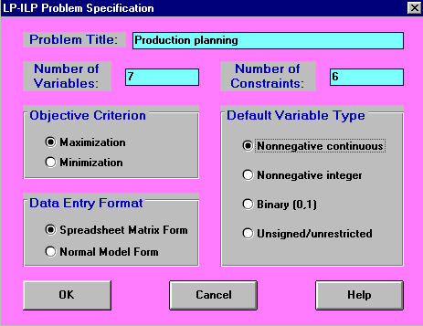
which sets up the input and then we have a spreadsheet type screen into which we enter the problem data, as below

There are a number of points to make:
We can show the problem in a more natural form (equation form) by using "Switch to Normal Model Form" to get:
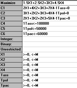
The solution to this problem is also shown below.
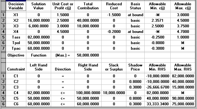
We can see that the optimal solution to the LP has value 58000 (£) and that Tass=82000, Tpol=50000, Tpac=60000, X1=0, X2=16000, X3=6000 and X4=0.
This implies that we only produce variants 2 and 3 (a somewhat surprising result in that we are producing none of variant 4 which had the highest profit per unit produced).
Referring back to the physical situation we can see that at the LP optimal we have 18,000 minutes of assembly time that is not used (Tass=82000 compared with a maximum time of 100000) but that all of the polishing and packing time is used.
For each constraint in the problem we also have a "Slack or Surplus" column. This column tells us, for a particular constraint, the difference between the left-hand side of the constraint when evaluated at the LP optimal (i.e. when evaluated with X1, X2, X3 and X4 taking the values given above) and the right-hand side of the constraint.
Constraints with a "Slack or Surplus" value of zero are said to be tight or binding in that they are satisfied with equality at the LP optimal. Constraints which are not tight are called loose.
A summary of the input to the computer for the second situation considered in the question (only limitation is on total time spent on all operations) is shown below.

which in equation form is:
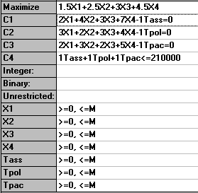
The solution to this problem is also shown below.
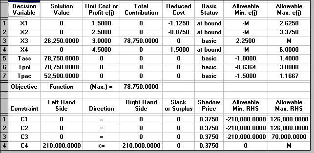
We can see that the optimal solution to the LP has value 78750 (£) and that Tass=78750, Tpol=78750, Tpac=52500, X1=0, X2=0, X3=26250 and X4=0.
This implies that we only produce variant 3.
Note here how much higher the associated profit is than before (£78750 compared with £58000, an increase of 36%!). This indicates that, however the allocation given before of 100,000; 50,000 and 60,000 minutes for assembly, polishing and packing respectively was arrived at it was a bad decision!
Solution - using Solver
Below we solve this LP with the Solver add-in that comes with Microsoft Excel.
If you click here you will be able to download an Excel spreadsheet called lp.xls that already has the LP we are considering set up.
Take this spreadsheet and look at Sheet A. You should see the problem we considered above set out as:

Here the values in cells B2 to B5 are how much of each variant we choose to make - here set to zero. Cells C6 to E6 give the total assembly/polishing and packing time used and cell F6 the total profit associated with the amount we choose to produce.
To use Solver in Excel do Tools and then Solver. In the version of Excel I am using (different versions of Excel have slightly different Solver formats) you will get the Solver model as below:
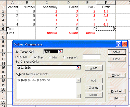
Here our target cell is F6 (ignore the use of $ signs here - that is a technical Excel issue if you want to go into it in greater detail) which we wish to maximise. We can change cells B2 to B5 - i.e. the amount of each variant we produce subject to the constraint that C6 to E6 - the total amount of assembly/polishing/packing used cannot exceed the limits given in C7 to E7.
In order to tell Solver we are dealing with a linear program click on Options in the Solver box and you will see:
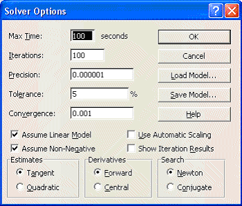
where both the 'Assume Linear Model' and 'Assume Non-Negative' boxes are ticked - indicating we are dealing with a linear model with non-negative variables.
Solving via Solver the solution is:

We can see that the optimal solution to the LP has value 58000 (£) and that Tass=82000, Tpol=50000, Tpac=60000, X1=0, X2=16000, X3=6000 and X4=0.
This implies that we only produce variants 2 and 3 (a somewhat surprising result in that we are producing none of variant 4 which had the highest profit per unit produced).
Referring back to the physical situation we can see that at the LP optimal we have 18,000 minutes of assembly time that is not used (Tass=82000 compared with a maximum time of 100000) but that all of the polishing and packing time is used.
For the second situation given in the question, where the only limitation is on the total time spent on all operations examine Sheet B in spreadsheet lp.xls
Invoking Solver in that sheet you will see:
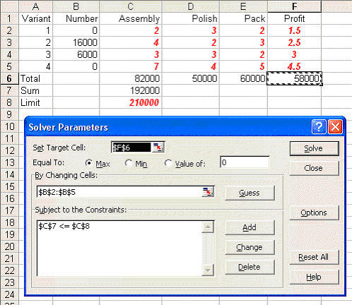
where cell C7 is the total amount of processing time used and the only constraint in Solver relates to that cell not exceeding the limit of 210000 shown in cell C8. Note here that if you check Options in Solver here you will see that both the 'Assume Linear Model' and 'Assume Non-Negative' boxes are ticked.
Solving we get:
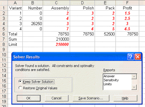
We can see that the optimal solution to the LP has value 78750 (£) and that Tass=78750, Tpol=78750, Tpac=52500, X1=0, X2=0, X3=26250 and X4=0.
This implies that we only produce variant 3.
Note here how much higher the associated profit is than before (£78750 compared with £58000, an increase of 36%!). This indicates that, however the allocation given before of 100,000; 50,000 and 60,000 minutes for assembly, polishing and packing respectively was arrived at it was a bad decision!
Problem sensitivity refers to how the solution changes as the data changes. Two issues are important here:
We deal with each of these in turn.
Robustness
Plainly, in the real world, data is never completely accurate and so we would like some confidence that any proposed course of action is relatively insensitive (robust) with respect to data inaccuracies. For example, for the production planning problem dealt with before, how sensitive is the optimal solution with respect to slight variations in any particular data item.
For example consider the packing time consumed by variant 3. It is currently set to exactly 2 minutes, i.e. 2.0000000. But suppose it is really 2.1, what is the effect of this on what we are proposing to do?
What is important here is what you might call "the shape of the strategy" rather than the specific numeric values. Look at the solution of value 58000 we had before. The shape of the strategy there was "none of variant 1 or 4, lots of variant 2 and a reasonable amount of variant 3". What we would like is that, when we resolve with the figure of 2 for packing time consumed by variant 3 replaced by 2.1, this general shape remains the same. What might concern us is if we get a very different shape (e.g. variants 1 and 4 only).
If the general shape of the strategy remains essentially the same under (small) data changes we say that the strategy is robust.
If we take Sheet A again, change the figure of 2 for packing time consumed by variant 3 to 2.1 and resolve we get:

This indicates that for this data change the strategy is robust.
Planning
With regard to planning we may be interested in seeing how the solution changes as the data changes (e.g. over time). For example for the production planning problem dealt with above (where the solution was of value 58000 involving production of variants 2 and 3) how would increasing the profit per unit on variant 4 (e.g. by 10 per cent to 4.95 by raising the price) impact upon the optimal solution.
Again taking Sheet A, making the appropriate change and resolving, we get:

indicating that if we were able to increase the profit per unit on variant 4 by 10 per cent to 4.95 it would be profitable to make that variant in the quantities shown above.
There is one thing to note here - namely that we have a fractional solution X3=1428.571 and X4=11428.57. Recall that we have a linear program - for which a defining characteristic is that the variables are allowed to take fractional values. Up to now for this production planning problem we had not seen any fractional values when we solved numerically - here we do. Of course in reality, given that the numbers are large there is no practical significance to these fractions and we can equally well regard the solution as being a conventional integer (non-fractional) solution such as X3=1429 and X4=11429.
Approach
In fact the approach taken both for robustness and planning issues is identical, and is often referred to as sensitivity analysis.
Given the LP package it is a simple matter to change the data and resolve to see how the solution changes (if at all) as certain key data items change.
In fact, as a by-product of using the simplex algorithm, we automatically get sensitivity information (e.g. the reduced cost information given on the LP output for the production planning problem):
However, interpreting simplex sensitivity information is somewhat complicated and so, for the purposes of this course, I prefer to approach sensitivity via resolving the LP. Those interested in interpreting the sensitivity information automatically produced by the simplex algorithm can find some information here.
Most large LP's are not entered directly into the computer in the same fashion as in our simple package. Instead an algebraic modelling language is used. A tutorial description of one of these modelling languages is available here. More about advanced LP can be found here.
Until the 1980's all packages for solving LP's relied upon variants of the simplex algorithm. However in 1984 Karmarkar published a new algorithm for LP, called an interior point method, which is completely different from the simplex algorithm.
Karmarkar's work has sparked an immense amount of LP research, both into interior point methods and into improving the simplex algorithm.
Since 1984 new commercial software products have appeared, e.g.
Both these products now include both simplex and interior point algorithms.
Let us consider the case where we have formulated some problem as an LP and we are thinking of solving it numerically. Can we find a computer package that has the capacity to solve our LP?
In terms of LP's the key factor is the number of constraints and a typical workstation/mainframe LP package (e.g. OSL (version 2)) has the capacity for 2 billion variables and 16 million constraints (excluding bounds on variables which are treated implicitly rather than explicitly).
However, these capacity limits vastly overstate what we could actually solve in real-life. To give you a rough idea of the state of the art the following results have been reported:
Code   Number of constraints  Number of variables  Time      Computer
OSL    105,000                155,000              4 hours   IBM 3090
       750                    12,000,000           27 mins   IBM 3090
Cplex  145                    1,000,000            6 mins    Cray Y-MP
       41,000                 79,000               3 mins    Cray 2
This is not to say that it is going to be impossible to solve very large LP's by simplex as there is a small chance that advanced LP theory might enable us to solve such problems (by decomposition or by taking advantage of any structure in the LP) but essentially we face a very difficult task.
Note here that the problem with solving very large LP's via simplex is not merely a matter of using a faster computer - the problem is theoretical in nature due to large LP's being degenerate (there is some evidence to suggest that for large LP's the solution time required when using simplex is approximately proportional to (number of constraints)2.4).
Problem areas where large LP's arise are:
The problem here is to determine where undersea cables and satellite circuits should be installed, when they will be needed, the number of circuits needed, cable technology, call routing, etc over a 19 year planning horizon (an LP with 28,000 constraints, 77,000 variables).
The problem is to plan US Army officer promotions (to Lieutenant, Captain, Major, Lieutenant Colonel and Colonel), taking into account the people entering and leaving the Army and training requirements by skill categories to meet the overall Army force structure requirements (an LP with 21,000 constraints and 43,000 variables).
The US Air Force Military Airlift Command (MAC) has a patient evacuation problem that can be modelled as a LP. They use this model to determine the flow of patients moved by air from an area of conflict to bases and hospitals in the continental United States. The objective is to minimise the time that patients are in the air transport system. The constraints are:
MAC have generated a series of problems based on the number of time periods (days). A 50 day problem consists of an LP with 79,000 constraints and 267,000 variables (solved in 10 hours).
The US Department of Defense Joint Chiefs of Staff have a logistics planning problem that models the feasibility of supporting military operations during a crisis.
The problem is to determine if different materials (called movement requirements) can be transported overseas within strict time windows.
The LP includes capacities at embarkation and debarkation ports, capacities of the various aircraft and ships that carry the movement requirements and penalties for missing delivery dates.
One problem (using simulated data) that has been solved had 15 time periods, 12 ports of embarkation, 7 ports of debarkation and 9 different types of vehicle for 20,000 movement requirements. This resulted in an LP with 20,500 constraints and 520,000 variables (solved in 75 minutes).
Many financial transactions can be modelled as LP's, e.g. bond arbitrage, switching between various financial instruments (bonds) so as to make money. Typical problems have approximately 1,000 constraints and 50,000 variables and can be solved in "real-time".
Here solving an LP is only the first stage in deciding crew schedules for commercial aircraft. The problem that has to be solved is actually an integer programming problem, the set partitioning problem. American Airlines has a problem containing 12,000,000 potential crew schedules (variables) - see OSL above. As such crew scheduling models are a key to airline competitive cost advantage these days (crew costs often being the second largest flying cost after fuel costs) we shall enlarge upon this problem in greater detail.
Within a fixed airline schedule (the schedule changing twice a year typically) each flight in the schedule can be broken down into a series of flight legs. A flight leg comprises a takeoff from a specific airport at a specific time to the subsequent landing at another airport at a specific time. For example a flight in the schedule from Chicago O'Hare to London Heathrow might have 2 flight legs, from Chicago to JFK New York and from JFK to Heathrow. A key point is that these flight legs may be flown by different crews.
Typically in a crew scheduling exercise aircraft types have been preassigned (not all crews can fly all types) so for a given aircraft type and a given time period (the schedule repeating over (say) a 2 week period) the problem becomes one of ensuring that all flight legs for a particular aircraft type can have a crew assigned. Note here that by crew we mean not only the pilots/flight crew but also the cabin service staff, typically these work together as a team and are kept together over a schedule.
As you probably know there are many restrictions on the hours that crews (pilots and others) can work. These restrictions can be both legal restrictions and union agreement restrictions. A potential crew schedule is a series of flight legs that satisfies these restrictions, i.e. a crew could successfully and legally work the flight legs in the schedule. All such potential crew schedules can have a cost assigned to them.
Hence for our American Airlines problem the company has a database with 12 million potential crew schedules. Note here that we stress the word potential. We have a decision problem here, namely out of these 12 million which shall we choose (so as to minimise costs obviously) and ensure that all flight legs have a crew assigned to them.
Typically a matrix type view of the problem is adopted, where the rows of the matrix are the flight legs and the columns the potential crew schedules, as below.
           Crew schedules
           1   2   3 etc ----->
Leg  A-B   0   1   1
     B-C   0   1   1
     C-A   0   0   1
     B-D   0   0   0
     A-D   1   0   0
     D-A   1   0   0
     etc
Here a 0 in a column indicates that that flight leg is not part of the crew schedule, a 1 that the flight leg is part of the crew schedule. Usually a crew schedule ends up with the crew returning to their home base, e.g. A-D and D-A in crew schedule 1 above. A crew schedule such as 2 above (A-B and B-C) typically includes as part of its associated cost the cost of returning the crew (as passengers) to their base. Such carrying of crew as passengers (on their own airline or on another airline) is called deadheading.
LP is used as part of the solution process for this crew scheduling problem for two main reasons:
Plainly there are people in the real world with large LP problems to solve. Informally what appears to be happening currently is that an increase in solution technology (advances in hardware, software and algorithms) is leading to users becoming aware that large problems can be tackled. This in turn is generating a demand for further improvements in solution technology.
Some other linear programming solution examples can be found here.