OR-Notes are a series of introductory notes on topics that fall under the broad heading of the field of operations research (OR). They were originally used by me in an introductory OR course I give at Imperial College. They are now available for use by any students and teachers interested in OR subject to the following conditions.
A full list of the topics available in OR-Notes can be found here.
Recall the production planning problem concerned with four variants of the same product which we formulated before as an LP. To remind you of it we repeat below the problem and our formulation of it.
A company manufactures four variants of the same product and in the final part of the manufacturing process there are assembly, polishing and packing operations. For each variant the time required for these operations is shown below (in minutes) as is the profit per unit sold.
                Assembly      Polish    Pack        Profit (£)
Variant 1       2             3         2           1.50
        2       4             2         3           2.50
        3       3             3         2           3.00
        4       7             4         5           4.50
Let:
xi be the number of units of variant i (i=1,2,3,4) made per year
Tass be the number of minutes used in assembly per year
Tpol be the number of minutes used in polishing per year
Tpac be the number of minutes used in packing per year
where xi >= 0 i=1,2,3,4 and Tass, Tpol, Tpac >= 0
(a) operation time definition
Tass = 2x1 + 4x2 + 3x3 +
7x4 (assembly)
Tpol = 3x1 + 2x2 + 3x3 + 4x4
(polish)
Tpac = 2x1 + 3x2 + 2x3 + 5x4
(pack)
(b) operation time limits
The operation time limits depend upon the situation being considered. In the first situation, where the maximum time that can be spent on each operation is specified, we simply have:
Tass <= 100000 (assembly)
Tpol <= 50000 (polish)
Tpac <= 60000 (pack)
In the second situation, where the only limitation is on the total time spent on all operations, we simply have:
Tass + Tpol + Tpac <= 210000 (total time)
Presumably to maximise profit - hence we have
maximise 1.5x1 + 2.5x2 + 3.0x3 + 4.5x4
which gives us the complete formulation of the problem.
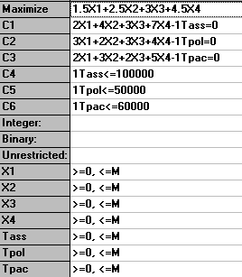
A summary of the input to the computer package for the first situation considered in the question (maximum time that can be spent on each operation specified) is shown below.

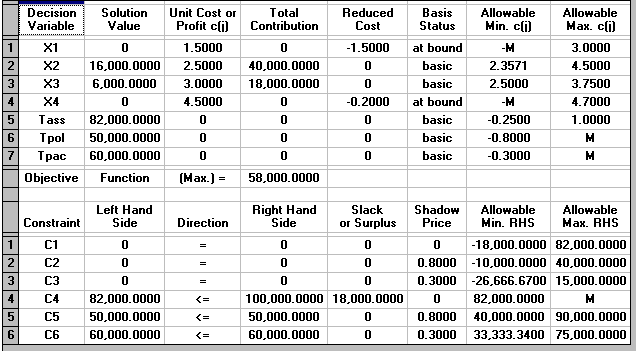
The solution to this problem is also shown below.

We can see that the optimal solution to the LP has value 58000 (£) and that Tass=82000, Tpol=50000, Tpac=60000, X1=0, X2=16000, X3=6000 and X4=0.
This then is the LP solution - but it turns out that the simplex algorithm (as a by-product of solving the LP) gives some useful information. This information relates to:
We deal with each of these in turn, and note here that the analysis presented below ONLY applies for a single change, if two or more things change then we effectively need to resolve the LP.
Currently X1=0, X2=16000, X3=6000 and X4=0. The Allowable Min/Max c(i) columns above tell us that, provided the coefficient of X2 in the objective function lies between 2.3571 and 4.50, the values of the variables in the optimal LP solution will remain unchanged. Note though that the actual optimal solution value will change.
In terms of the original problem we are effectively saying that the decision to produce 16000 of variant 2 and 6000 of variant 3 remains optimal even if the profit per unit on variant 2 is not actually 2.5 (but lies in the range 2.3571 to 4.50).
Similar conclusions can be drawn about X1, X3 and X4.
In terms of the underlying simplex algorithm this arises because the current simplex basic solution (vertex of the feasible region) remains optimal provided the coefficient of X2 in the objective function lies between 2.3571 and 4.50.
Hence we have the table
Variable                             X1      X4
Opportunity Cost                     1.5     0.2
New value (= or >=)                  X1=A    X4=B
                                  or X1>=A   X4>=B
Estimated objective function change  1.5A    0.2B
The objective function will always get worse (go down if we have a maximisation problem, go up if we have a minimisation problem) by at least this estimate. The larger A or B are the more inaccurate this estimate is of the exact change that would occur if we were to resolve the LP with the corresponding constraint for the new value of X1 or X4 added.
Hence if exactly 100 of variant one were to be produced what would be your estimate of the new objective function value?
Note here that the value in the Reduced Cost column for a variable is often called the "opportunity cost" for the variable.
Note here than an alternative (and equally valid) interpretation of the reduced cost is the amount by which the objective function coefficient for a variable needs to change before that variable will become non-zero.
Hence for variable X1 the objective function needs to change by 1.5 (increase since we are maximising) before that variable becomes non-zero. In other words, referring back to our original situation, the profit per unit on variant 1 would need to need to increase by 1.5 before it would be profitable to produce any of variant 1. Similarly the profit per unit on variant 4 would need to increase by 0.2 before it would be profitable to produce any of variant 4.
Hence we can form the table
Constraint                        Assembly    Polish    Pack
Opportunity Cost (ignore sign)    0           0.80      0.30
Change in right-hand side         a           b         c
Objective function change         0           0.80b     0.30c
Lower limit for right-hand side   82000       40000     33333.34
Current value for right-hand side 100000      50000     60000
Upper limit for right-hand side   -           90000     75000
For example for the polish constraint, provided the right-hand side of that constraint remains between 40000 and 90000 the objective function change will be exactly 0.80[change in right-hand side from 50000].
The direction of the change in the objective function (up or down) depends upon the direction of the change in the right-hand side of the constraint and the nature of the objective (maximise or minimise).
To decide whether the objective function will go up or down use:
Hence
The value in the column headed Shadow Price for a constraint is often called the "marginal value" or "dual value" for that constraint.
Note that, as would seem logical, if the constraint is loose the shadow price is zero (as if the constraint is loose a small change in the right-hand side cannot alter the optimal solution).
Note here that, as mentioned above, the analysis given above relating to:
is only valid for a single change. If two (or more) changes are made the situation becomes more complex and it becomes advisable to resolve the LP.
Consider the linear program:
maximise
3x1 + 7x2 + 4x3 + 9x4
subject to
x1 + 4x2 + 5x3 + 8x4 <= 9    (1)
x1 + 2x2 + 6x3 + 4x4 <= 7    (2)
xi >= 0 i=1,2,3,4
Solve this linear program using the computer package.
Solving the problem using the package the solution is:
Reading from the printout given above we have:
Note that we can, if we wish, explicitly enter the four constraints xi>=0 i=1,2,3,4. Although this is unnecessary (since the package automatically assumes that each variable is >=0) it is not incorrect. However, it may alter some of the solution figures - in particular the Reduced Cost figures may be different. This illustrates that such figures are not necessarily uniquely defined at the linear programming optimal solution.