OR-Notes are a series of introductory notes on topics that fall under the broad heading of the field of operations research (OR). They were originally used by me in an introductory OR course I give at Imperial College. They are now available for use by any students and teachers interested in OR subject to the following conditions.
A full list of the topics available in OR-Notes can be found here.
You will recall that in formulating linear programs (LP's) and integer programs (IP's) we tried to ensure that both the objective and the constraints were linear - that is each term was merely a constant or a constant multiplied by an unknown (e.g. 5x is a linear term but 5x² a nonlinear term). Unless all terms were linear our solution algorithms (simplex/interior point for LP and tree search for IP) would not work.
Here we will look at problems which do contain nonlinear terms. Such problems are generally known as nonlinear programming (NLP) problems and the entire subject is known as nonlinear programming.
The mathematics of nonlinear programming is very complex and will not be considered here.
We will illustrate nonlinear programming with the aid of a number of examples solved using the package. A restricted capacity free copy of some software from Lindo Systems for solving nonlinear programs is available here. Another package is available here.
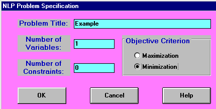
Consider the following nonlinear program:
minimise     x(sin(3.14159x))
subject to   0 <= x <= 6
Here we have only one nonlinear term x(sin(3.14159x)) which is in the objective which we are trying to minimise.
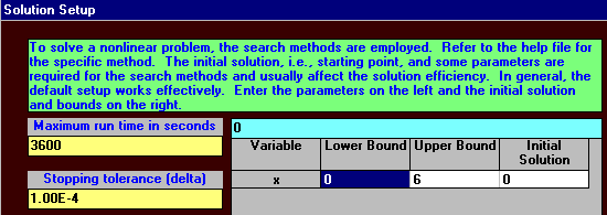
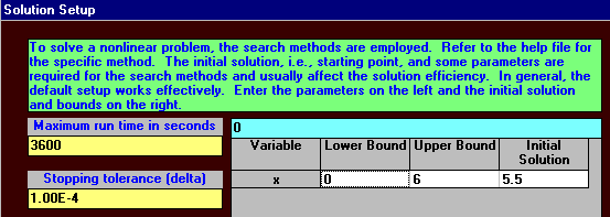
Inputting this example problem to the package we have

with the solution setup being:
and the solution itself being:
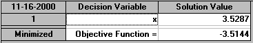
In other words the package has decided the solution is x=3.5287 with the associated objective function value being -3.5144. The only problem is that this is incorrect! To see this suppose that we plot on a graph the objective function x(sin(3.14159x)) for values of x from 0 to 6. We get the graph shown below.
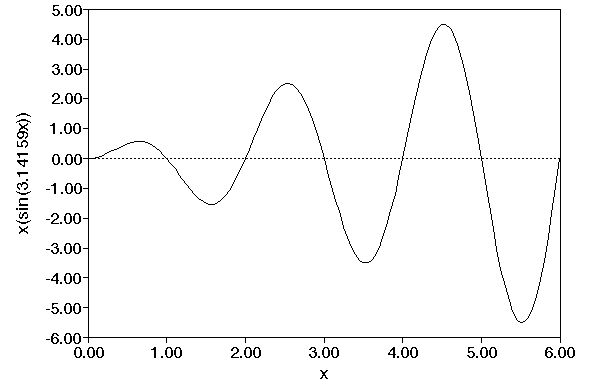
Note that in this graph the minimum value of x(sin(3.14159x)) occurs at around x=5.5, i.e. the package solution of x=3.5287 is wrong!
In fact the package is working correctly. The problem lies not in the package but is inherent in the underlying mathematical difficulties of solving nonlinear programs. In the diagram above there are many local optima (minima in this case) - that is points at the bottom of some portion of the graph. But only one global optimum (minimum in this case). In fact we can see that the solution produced by the package (x=3.5287) is a local optimum.
Obviously we would like to have some general solution method for nonlinear programs (such as we have for LP's and IP's) that always produces the global optimum for any nonlinear program. No such solution method exists - a local optimum is produced and we cannot be sure (in all cases) whether this is the global optimum or not. One way to try and see whether we have the global optimum is to resolve (once or more) from a user-supplied starting point (initial solution in package terminology) to see if we get the same solution. If we do then this raises confidence that we have actually found the global optimum.
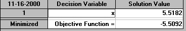
For example resolving the problem given above with a user-supplied initial solution for x of 5.5 gives the global optimum of x=5.5182 (see below).
In general we can say that nonlinear programs are difficult to solve and suffer from the fact that it is difficult to be sure whether the global optimum has been found or not. In addition the computation time consumed in reaching a solution to a nonlinear program can be high (much higher than for a similar sized LP for example).
The above example had a nonlinear objective, but no nonlinearities in the constraints, indeed the only restriction was a bound on the single decision variable.
Consider a more difficult example:
maximise 2x1 + x2 - 5loge(x1)sin(x2)
subject to
x1x2 <= 10
| x1 - x2 | <= 2
0.1 <= x1 <= 5
0.1 <= x2 <= 3
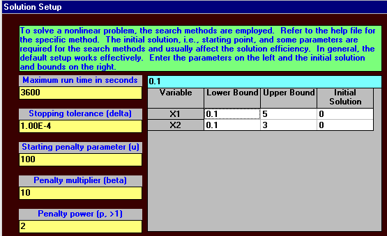
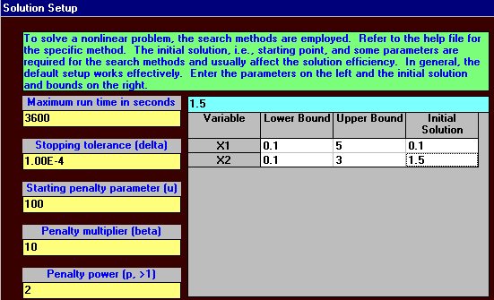
Here we have a nonlinear objective and nonlinear constraints. Using the package we have the input:

and taking the default "Solution Setup" as below
we get the solution:

i.e. x1=3.3340 and x2=2.9997 with an associated objective function value of 8.8166
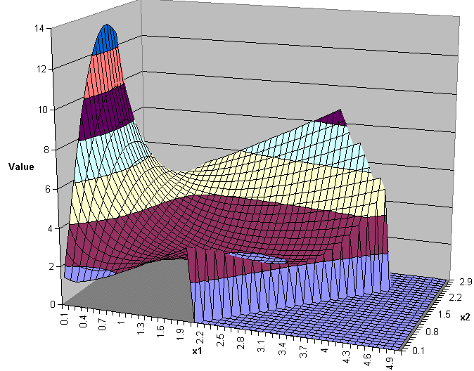
However a three-dimensional plot of the problem gives:
 :
:
and it clear from this there there are values of x1 and x2 that exceed the supposed maximum objective function value of 8.8166 given by the package.
Again changing the "Solution Setup" screen as below to provide an intelligent initial solution:
 #
#
and solving we get:
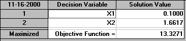
which seems much more satisfactory.
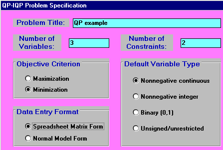
A quadratic program is a nonlinear program where:
For an example quadratic programming problem consider the problem shown below.
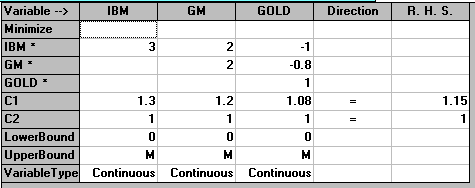
This is a portfolio investment problem where we want the amount to invest each of three assets (IBM, GM and GOLD) where we adjust the amounts invested to achieve a desired return at minimum risk (defined as the variance of the return). This problem is a portfolio optimisation problem, more about portfolio optimisation (but at a research level rather than at a basic teaching level) can be found here.
The problem is:

You can see why this is a quadratic program, although here we have no linear terms in or particular objective function all terms are products of just two variables. Moreover the constraints are linear. This problem is entered via the "Quadratic Programming" module in the package as below:
with the solution being:
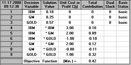
i.e. IBM=0.18, GM=0.25 and GOLD=0.57
The reason for using the quadratic programming module in the package, rather than the nonlinear programming module we used before is that as we are dealing with a quadratic program special algorithms exists that can, in certain circumstances, guarantee to find the optimal solution. This contrasts with general nonlinear programming as we considered it above where, as we demonstrated, the package failed to find the optimal (best) solution without some inspired guesswork on our part with regard to an initial solution.
More about nonlinear programming using separable programming can be found here.