OR-Notes are a series of introductory notes on topics that fall under the broad heading of the field of operations research (OR). They were originally used by me in an introductory OR course I give at Imperial College. They are now available for use by any students and teachers interested in OR subject to the following conditions.
A full list of the topics available in OR-Notes can be found here.
Whilst it is conventional to deal numerically with network diagrams using the standard dynamic programming algorithm considered before there are advantages to considering how to analyse such diagrams using linear programming (LP).
Below we repeat the (activity on node) network diagram for the problem we considered before. However note that we have now added a dummy activity (12) with a completion time of zero to represent the end of the project. This just makes the calculations we have to do easier to follow
Linear programming is a standard technique that involves formulating a problem using:
The word linear implies that all terms involved in the formulation must be linear terms (i.e. either a constant or a constant multiplied by an unknown).
In order to analyse the network given above by linear programming let xi (>=0) represent the time at which we start activity i. This time is our choice and hence is a decision variable. Note here that:
Considering the precedence relationship between activity 1 and activity 3 it is clear that we must have
x3 >= x1 + 6
i.e. the starting time for activity 3 must be at least as great as the starting time for an immediate predecessor activity plus the completion time for this predecessor activity. Note that we do not put x3 = x1 + 6 here. This is because the inequality (>=) gives us more flexibility than the equality (=).
By exactly the same logic we must also have
x4 >= x2 + 2
x5 >= x3 + 3
x6 >= x4 + 2
Now activity 7 has two immediate predecessor activities so we need two constraints:
x7 >= x5 + 4
x7 >= x6 + 1
Continuing we have that the remaining constraints are:
x8 >= x7 + 1
x9 >= x8 + 6
x10 >= x8 + 6
x11 >= x9 + 3
x11 >= x10 + 1
x12 >= x11 + 1
Our objective is (as before) to complete the project in the minimum possible time i.e.
minimise x12
Hence we have that a complete linear programming formulation of the problem of deciding the start time for each activity so as to respect the precedence relationships and complete the project in the minimum possible time is given by:
minimise x12
subject to
x3 >= x1 + 6
x4 >= x2 + 2
x5 >= x3 + 3
x6 >= x4 + 2
x7 >= x5 + 4
x7 >= x6 + 1
x8 >= x7 + 1
x9 >= x8 + 6
x10 >= x8 + 6
x11 >= x9 + 3
x11 >= x10 + 1
x12 >= x11 + 1
xi >= 0 i=1,2,...,12
This linear program (LP) can be solved using the package as below.
The input needed to enter the model is:
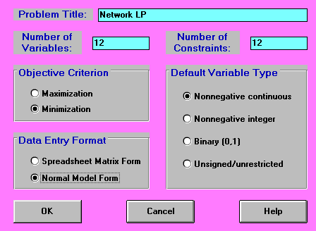
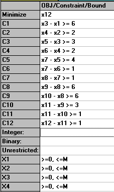
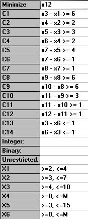
The model is entered (using Normal Model Form above) in a natural way as shown (in part) below:
The solution is given by:
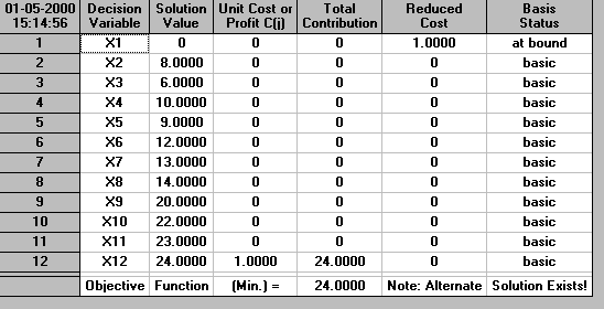
So we can see immediately that the minimum possible completion time is 24 (weeks). As we would expect this is exactly the same as calculated previously using the dynamic programming algorithm. However note that there are differences between what we obtain from linear programming and what we previously obtained by dynamic programming:
In fact we can, relatively easily, determine which activities are critical and which are non-critical. This is accomplished by adding the constraint x12=24 (the determined minimum completion time) to the above linear program and then solving, for each activity i the two LP's
For example solving these two LP's with activity 5 results in the minimum value of x5 being 9 and the maximum value of x5 being 9, indicating that activity 5 is critical and must be started at time 9 if the project is to be completed in 24 weeks.
By contrast solving these two LP's with activity 10 results in the minimum value of x10 being 20 and the maximum value of x10 being 22, indicating that activity 10 is non-critical and can be started anytime between 20 and 22 if the project is to be completed in 24 weeks.
So far we have essentially merely duplicated via linear programming what we could already do via dynamic programming. In fact reflect here that using dynamic programming we could work out the critical path/activities without a computer. Using linear programming this not be possible (and even if I taught you how to solve linear programs without a computer it would be much more time-consuming and complicated). The real benefit of using linear programming comes if we add additional constraints into the problem. We deal with a number of typical additional constraints below. In all cases considered below incorporating these conditions in a general way into the network for solution via dynamic programming is impossible. This illustrates that using LP can provide us with the ability to impose upon our network more conditions, reflecting the reality of the project. However this extra ability comes at a price, LP's are more difficult to formulate and more time-consuming to solve.
In the notation below A and B are two activities with completion times a and b.
Suppose that for some reason we had a time window on the time at which some activity could start. For example we might wish (e.g. for contractual reasons) to start activity 3 between time 4 and time 8. This can be achieved by adding to the LP the constraint 4 <= x3 <= 8. In a similar fashion we can also restrict finish times (since finish time = start time + completion time), e.g. restricting the finish time for activity 3 to be between 6 and 10 is achieved using 6 <= x3 + 3 <= 10
Suppose that for some reason we wanted activities 3 and 6 to start at exactly the same time. In other words we require x3 = x6. With the LP we could easily deal with this requirement by adding the constraint x3 = x6 to the LP.
Suppose now that for some reason we wanted activities 3 and 6 to start at "roughly" the same time, where by roughly here we will mean within one week of each other. In other words we require |x3 - x6| <= 1. By making use of the LP formulation of the problem given above we can easily incorporate |x3 - x6| <= 1. Whilst this constraint is nonlinear (because of the modulus sign) it is equivalent to adding to our original LP the two linear constraints:
The additional constraints added to the original LP are shown (in part) below:

and the solution is:
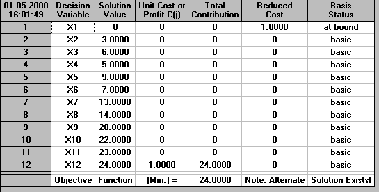
showing that we can still complete the project in 24 weeks with this new restriction.
Suppose now we add the additional restriction that |x4 - x5| <= 1. Can we still complete the project in 24 weeks?
Adding the two constraints x4 - x5 <= 1 and x5 - x4 <= 1 to the LP we had previously (which already incorporated the restriction that |x3 - x6| <= 1) and solving reveals that the problem is now infeasible. In other words with this new restriction added there are no values for the variables that can satisfy the constraints.
Whilst for a number of the cases given above we may, for this small project network, be able to see what happens by eye. However if we impose a number of these additional constraints then it becomes much more difficult to gauge the effect by eye. For example what would be the effect upon the project of insisting that:
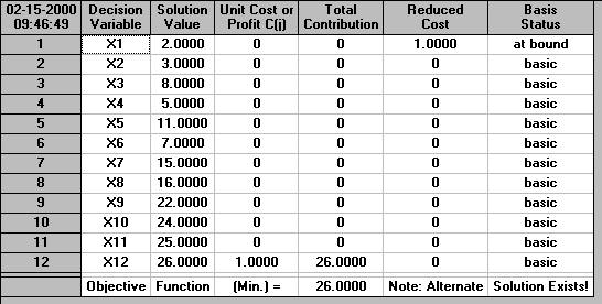
The solution using the package is shown below. It can be seen that in this case the minimum possible project completion time is 26 weeks, an increase of 2 weeks from before. This means that we have explicitly seen the effect of imposing our extra requirements upon the project.
We shall return to using linear programming in the context of network analysis when we deal with cost/time tradeoff.