
OR-Notes are a series of introductory notes on topics that fall under the broad heading of the field of operations research (OR). They were originally used by me in an introductory OR course I give at Imperial College. They are now available for use by any students and teachers interested in OR subject to the following conditions.
A full list of the topics available in OR-Notes can be found here.
Recall from queueing theory that in essence all queuing systems can be broken down into individual sub-systems consisting of entities queuing for some activity (as shown below).

Typically we can talk of this individual sub-system as dealing with customers queuing for service. To analyse this sub-system we need information relating to:
Note here that integral to queuing situations is the idea of uncertainty in, for example, interarrival times and service times. This means that probability and statistics are needed to analyse queuing situations.
Whilst queueing theory can be used to analyse simple queueing systems more complex queueing systems are typically analysed using simulation (more accurately called discrete-event simulation). Precisely what discrete-event simulation is will become clearly below.
In OR we typically deal with discrete-event simulation. Note here however that the word simulation has a wider meaning. For example you may have heard of aircraft simulators which reproduce the behaviour of an aircraft in flight, but in reality one never leaves the ground. These are used for training purposes. You may have taken part in a business game simulation in which you were in charge of an imaginary company and the results for your company (sales made, profit, etc) were generated by a computer in some manner. These are often called business simulations.
More about simulation can be found here and here.
To illustrate discrete-event simulation let us take the very simple system below, with just a single queue and a single server.

Suppose that customers arrive with interarrival times that are uniformly distributed between 1 and 3 minutes, i.e. all arrival times between 1 and 3 minutes are equally likely. Suppose too that service times are uniformly distributed between 0.5 and 2 minutes, i.e. any service time between 0.5 and 2 minutes is equally likely. We will illustrate how this system can be analysed using simulation.
Conceptually we have two separate, and independent, statistical distributions. Hence we can think of constructing two long lists of numbers - the first list being interarrival times sampled from the uniform distribution between 1 and 3 minute, the second list being service times sampled from the uniform distribution between 0.5 and 2 minutes. By sampled we mean that we (or a computer) look at the specified distribution and randomly choose a number (interarrival time or service time) from this specified distribution. For example in Excel using 1+(3-1)*RAND() would randomly generate interarrival times and 0.5+(2-0.5)*RAND() would randomly generate service times.
Suppose our two lists are:
Interarrival times      Service times
      1.9                    1.7
      1.3                    1.8
      1.1                    1.5
      1.0                    0.9
      etc                    etc
where to ease the processing we have chosen to work one decimal place.
Suppose now we consider our system at time zero (T=0), with no customers in the system. Take the lists above and ask yourself the question: What will happen next?
The answer is that after 1.9 minutes have elapsed a customer will appear. The queue is empty and the server is idle so this customer can proceed directly to being served. What will happen next?
The answer is that after a further 1.3 minutes have elapsed (i.e. at T=1.9+1.3=3.2) the next customer will appear. This customer will join the queue (since the server is busy).What will happen next?
The answer is that at time T=1.9+1.7=3.6 the customer currently being served will finish and leave the system. At that time we have a customer in the queue and so they can start their service (which will take 1.8 minutes and hence end at T=3.6+1.8=5.4).What will happen next?
The answer is that 1.1 minutes after the previous customer arrival (i.e. at T=3.2+1.1=4.3) the next customer will appear. This customer will join the queue (since the server is busy).What will happen next?
The answer is that after a further 1.0 minutes have elapsed (i.e. at T=4.3+1.0=5.3) the next customer will appear. This customer will join the queue (since there is already someone in the queue), so now the queue contains two customers waiting for service. What will happen next?
The answer is that at T=5.4 the customer currently being served will finish and leave the system. At that time we have two customers in the queue and assuming a FIFO queue discipline the first customer in the queue can start their service (which will take 1.5 minutes and hence end at T=5.4+1.5=6.9)What will happen next?
The answer is that ...... etc and we could continue in this fashion if we so wished (had the time and energy!). Plainly the above process is best done by a computer.
To summarise what we have done we can construct the list below:
Time T     What happened
 1.9       Customer appears, starts service scheduled to end at T=3.6
 3.2       Customer appears, joins queue
 3.6       Service ends
           Customer at head of queue starts service, scheduled to end at T=5.4
 4.3       Customer appears, joins queue
 5.3       Customer appears, joins queue
 5.4       Service ends
           Customer at head of queue starts service, scheduled to end at T=6.9
 etc
You can hopefully see from the above how we are simulating (artificially reproducing) the operation of our queuing system. Simulation, as illustrated above, is more accurately called discrete-event simulation since we are looking at discrete events through time (customers appearing, service ending). Here we were only concerned with the discrete points T=1.9,3.2,3.6,4.3,5.3,5.4,etc
Once we have done a simulation such as shown above then we can easily calculate statistics about the system - for example the average time a customer spends queueing and being served (the average time in the system). Here two customers have gone through the entire system - the first appeared at time 1.9 and left the system at time 3.6 and so spent 1.7 minutes in the system. The second customer appeared at time 3.2 and left the system at time 5.4 and so spent 2.2 minutes in the system. Hence the average time in the system is (1.7+2.2)/2 = 1.95 minutes.
We can also calculate statistics on queue lengths - for example what is the average queue size (length). Here the queue is of size 0 from T=0 to T=3.2, of size 1 from T=3.2 to 3.6, of size 0 from T=3.6 to T=4.3, of size 1 from T=4.3 to T=5.3, of size 2 from T=5.3 to T=5.4. Hence the time-weighted average queue size is:
[0(3.2-0)+1(3.6-3.2)+0(4.3-3.6)+1(5.3-4.3)+2(5.4-5.3)]/5.4 = 0.296
Note here however how the above calculations (both for average time in the system and average queue size) took into account the system when we first started - when it was completely empty. This is probably biasing (rendering inaccurate) the statistics we are calculating and so it is common in simulation to allow some time to elapse (so the system "fills up") before starting to collect information for use in calculating summary statistics.
In simulation statistical (and probability) theory plays a part both in relation to the input data and in relation to the results that the simulation produces. For example in a simulation of the flow of people through supermarket checkouts input data like the amount of shopping people have collected is represented by a statistical (probability) distribution and results relating to factors such as customer waiting times, queue lengths, etc are also represented by probability distributions. In our simple example above we also made use of a statistical distribution - the uniform distribution.
There are a number of problems relating to simulation models:
Once we have the model we can use it to:
Which of these factors (or combination of factors) will be the best choice to increase output. Note here that any change might reduce congestion at one point only to increase it at another point so we have to bear this in mind when investigating any proposed changes.
Special purpose computer languages have been developed to help in writing simulation programs (e.g. SIMSCRIPT) as have pictorial based languages (using entity-cycle diagrams) and interactive program generators. A comparatively recent development in simulation are packages which run with animation - essentially on screen one sees a representation of the system being simulated and objects moving around in the course of the simulation. Details of packages for simulation can be found here and here.
Simulation began to be applied to management situations in the late 1950's to look at problems relating to queuing and stock control. Monte-Carlo simulation was used to model the activities of facilities such as warehouses and oil depots. Queuing problems (e.g. supermarket checkouts) were also modelled using Monte-Carlo simulation. The phrase "Monte Carlo" derives from the well-known gambling city of Monte Carlo on the Mediterranean in Monaco. Just as in roulette we get random numbers produced by a roulette wheel when it is spun, so in Monte Carlo simulation we make use of random numbers generated by a computer.
The advantages of using simulation, as opposed to queuing theory, are:
One disadvantage of simulation is that it is difficult to find optimal solutions, unlike linear programming for example where we have an algorithm which will automatically find an optimal solution. The only way to attempt to optimise using simulation is to:
Large amounts of computer time can be consumed by this process.
Consider the queueing system below where we have two parts X and Y that are being assembled together. Before assembly can take place on Machine 3 both X and Y must undergo some processing on Machines 1 and 2 respectively. After assembly (one X part and one Y part going to make up an assembled item) further processing needs to take place on Machine 4 before the assembled item is completed. Obviously if a machine is busy then the parts/assembled items must wait for processing in the appropriate queue.
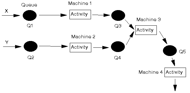
We shall analyse this system using the simulation module in the package.
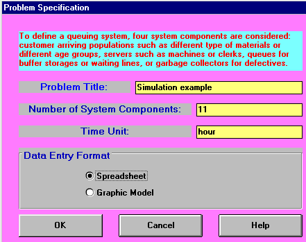
The initial package input screen is shown below. We have 11 components as there are 2 items being processed (X and Y), 5 queues and 4 activities (so 2+5+4=11 components).
We enter the names of each of the 11 components and their types as below:
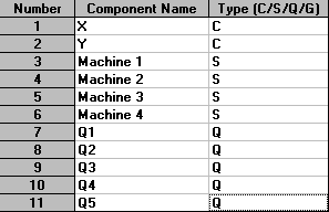
Here X and Y are the customers flowing through the system, so are designated type C; the machines are servicing these customers and so are designated type S; and the queues are designated type Q.
The initial part of the input is shown below.
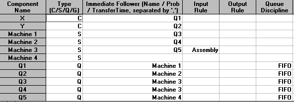
The "Immediate Follower" column is used to define how customers (X and Y in this case) flow thorough the system. Here X, as it enters the system, first goes to Q1, so that is its immediate follower above. Q1 is followed by Machine 1 and Machine 1 in turn is followed by Q3. Q3 is followed by Machine 3 and Machine 3 is followed by Q5 which is followed by Machine 4.
The "Input Rule" column is used to tell each server how to select a customer from the preceding queues. This column is only of significance when a server has more than one queue immediately preceding it. For our example this only occurs at Machine 3, where we have Q3 contain X parts and Q4 containing Y parts. The use of the word "Assembly" as the input rule for Machine 3 therefore says that one of each part must be available in Q3 and Q4 before the Machine 3 activity can start.
For all queues we have specified the queue discipline as FIFO (first-in first-out) meaning that parts are processed in the order in which they arrive in the queues.
The second part of the input is shown below.
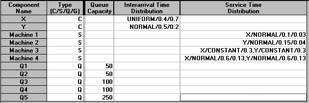
We have defined queue capacities above. Once a queue is full then the preceding activity cannot pass on a part (customer) until there is space available in the queue.
For the customers (X and Y) we need to specify an interarrival time distribution. Here we have assumed that X parts have interarrival times which are uniformly distributed between 0.4 and 0.7 hours. Y parts have interarrival times that are normally distributed with mean 0.5 hours and standard deviation 0.2 hours.
For the servers (Machines 1 to 5) we need to specify the service time distribution - for the parts that they process. Here Machine 1 processes X parts with a service time that is normally distributed with mean 0.1 hours and standard deviation 0.03 hours. Machine 2 processes Y parts with a service time that is normally distributed with mean 0.15 hours and standard deviation 0.04 hours. Machine 3 is the machine that assembles parts X and Y together so above we have specified it processes both parts with the same service time distribution (here a constant processing time of 0.3 hours).
Finally Machine 4 processes the assembled part and, because we cannot be sure what our particular package calls this assembled part (X or Y ?), we have specified the processing time for both parts as the same - here normally distributed with mean 0.6 hours and standard deviation 0.13 hours. This is just a limitation imposed by the (cheap) package we are using. More expensive simulation packages enable us to specify the system more exactly.
A graphical representation of the system, produced by the package, can be seen below.

The initial screen for the package solution is shown below.
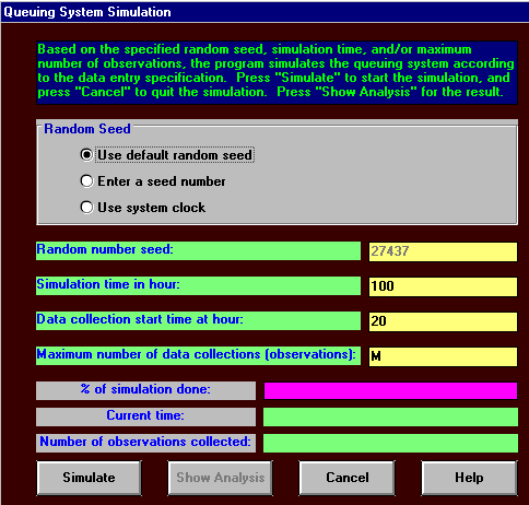
Here we have chosen to simulate for 100 hours. This does not mean we must wait for 100 hours of our life before we get any results! Rather this is 100 hours of time within the situation we are considering, i.e. internal simulation model time T in terms of the notation for the simple example we considered previously. It can be seen above that we will not start data collection (collecting data for statistics like average time in the system, average queue sizes, etc) until after 20 hours have elapsed. This is to allow the system to "fill up"
The initial package output is shown below.
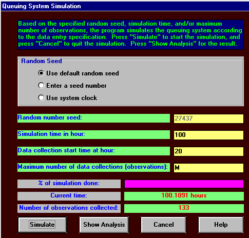
It can be seen that over the timespan for which we collected data, from T=20 to the end of the simulation, we have 133 observations to analyse. The simulation ended at T=101.1091, whereas we actually specified we wished to simulate for 100 hours. The reason for this is that the package runs until:
It then stops - here the first event necessitating a change in the system occurred at T=101.1091
The analysis produced by the package as a result of this simulation is shown below.
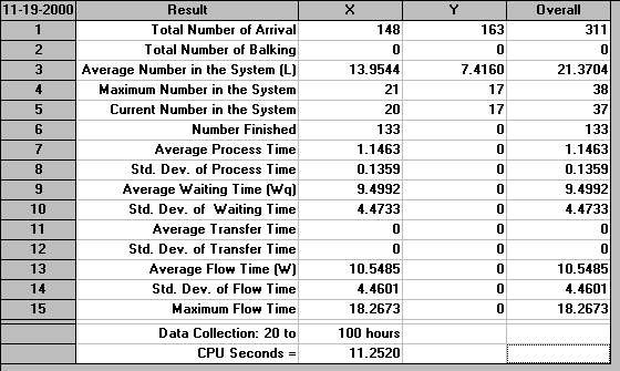
It can be seen that 148 X parts and 163 Y parts arrived in the system. The average (time-weighted) number in the system for X was 13.9544 and for Y was 7.4160. 133 items have been finished (assembled from X and Y and processed on Machine 4). It can be seen above that the package has designated these as X items. Hence we need to concentrate on X - the statistics above for X will refer to the flow through the system of X parts as they turn into assembled items and are eventually passed out of the system. Indeed this is why many of the statistics above for Y are given as zero.
The average process time, time spent processing a X part as it flows through the system is 1.1463 hours with a standard deviation of 0.1359 hours. At first sight it might appear odd as to how 133 items could have been completed if they required an average of 1.1463 processing hours each, a total of 133(1.1463) = 152.5 hours - far exceeding the 80 hours for which we collected data. The answer here lies in the nature of the system - processing is occurring simultaneously on different machine at the same point in time. Considering our diagram above of the system we are simulating, at any one time Machines 1, 3 and 4 can be processing X items - so over the 80 hours for which we collect data we could have at most 3(80)=240 processing hours.
The average waiting time experienced by a X part is 9.4992 hours with a standard deviation of 4.4733 hours. Theoretically the average processing time and the average waiting time (here 1.1463+9.4992 = 10.6455) should add to the average flow time (given above as 10.5485). Here there is a slight discrepancy due to the way the package internally keeps track of parts as they move through the system.
Information as to the utilisation of our servers (machines) is as below.

Once again the package shows its weaknesses by reporting a utilisation for Machine 4 of 100.24%, a seeming impossible figure. The package makes an error here because in calculating this figure it fails to distinguish between the actual end of the simulation, at time T=101.1091 and the desired end time of T=100. As far as I can see (although I may be wrong) the package calculates utilisation for Machine 4 using utilisation =100(time Machine 4 in use between T=20 and T=101.1091)/(time between T=20 and T=100)%. This can plainly exceed 100%, and does above!
Irrespective of this it is clear that Machine 4 is by far the most utilised machine and is hence a bottleneck in terms of the total system output.
Wee can also produce an analysis of the queues, as below.

Here Q5 is the largest queue, confirming our observation above that Machine 4 is the bottleneck in the production process.
As well as the above tables of numbers we can also produce graphical analysis, as below for example.
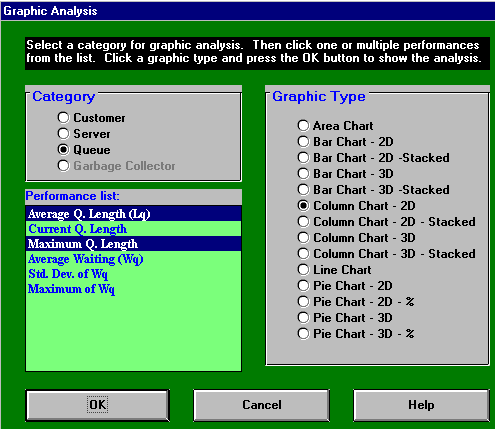
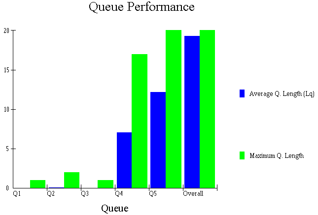
Producing graphical analyses is common in discrete-event simulation. It often enables us to get a clearer picture of the system and how it is performing than we would get by just staring at tables of numbers.
Once we have a simulation model for a system, such as above, then using it can give us useful insight into the behaviour of the system. Real-life systems can be complex with many interactions and it can be difficult, given statistical variations in processing and arrival times, queue capacities, etc to understand the entire system without the numerical insight provided by simulation.
In our system above, for example, it has become clear that Machine 4 is a bottleneck in terms of the overall production output. We might therefore be interested in seeing how we can improve the system, i.e. we want to explore changes to the system numerically using the simulation model we have constructed.
Examining our simulation situation, as below, one option here is to change the queue discipline for Q5, which is the queue just before Machine 4, the bottleneck.

Suppose we change that queue discipline from FIFO, the current discipline, to (in package terminology) MaxWorkDone - choose the next item for processing to be the one that has had the maximum work (processing) carried out on it already. The results of this are shown below.

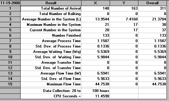
Comparing this output with the output we had before it can be seen that we finish exactly the same number of items. This is as we might expect as the processing times on Machine 4, for which we have changed the queue discipline for item choice, are NOT associated with the items chosen but (conceptually) are taken from a predefined list of processing times - as in our simple example above. Hence changing the order in which we choose items for processing on Machine 4 does not make any difference to the total number completed. What it does affect however is the flow time. Now the average flow time is given as 6.5941 hours, before it was 10.5485 hours. Conceptually individual items are spending less time in the system on average, although the total system output is unchanged.
One option we might explore to try and achieve more output is to get another Machine 4. Two machines at that point in the production system should enable us to substantially increase output. Indeed, since Machine 4 is the bottleneck common sense might well say that two machines would enable us to DOUBLE production. Do you agree? Would two machines enable us to double production or not? If not by how much would you estimate production would increase?
We can investigate this situation numerically using our simulation model. Focusing on just the final portion of our production system the situation now is:
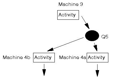
where Q5 feeds both machines (designated as 4a and 4b).
The package input is as below.
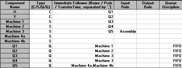
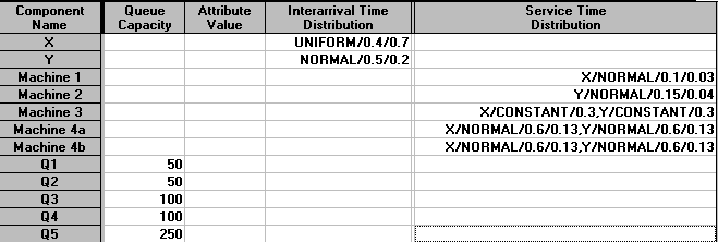
with the graphical model being:

The output, after simulating for the same time period as before, is:
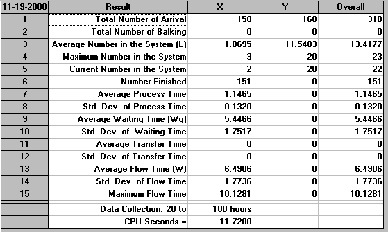


It can be seen that our expectation as to doubled production is way off the mark - according to our results we have increased production from the 133 items (approximately 133/80 = 1.7 items per hour) we had before to 151 items now (approximately 151/80 = 1.9 items per hour). This is an increase of only 0.2 items per hour (i.e. 100(0.2)/1.7= 11.8%). This is far from a doubling of production! How can we explain this?
Well perhaps the problem is that we have not simulated for long enough. Above we were producing 151 items in (approximately) 80 hours, i.e. 151/80 = 1.9 items per hour. Let us see what happens if we simulate for ten times as long (say for 1000 hours, where data collection starts after 200 hours). The output is shown below - production in (approximately) 800 hours is 1448 items, i.e. 1.8 items per hour.
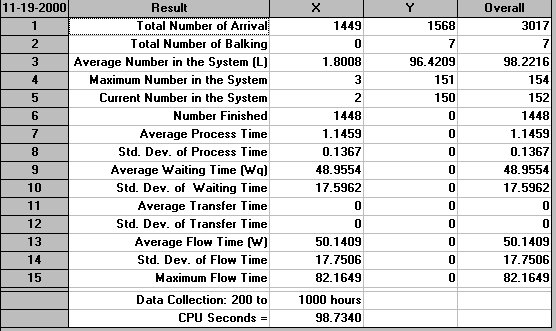
It is clear from simulating for longer that the effect we are seeing, having two Machine 4's does not double production is real. But why?
The simple answer is that this situation is common in simulation - linked systems of queues and activities, such as we have here, are notoriously difficult to analyse in terms of common sense. Instead a detailed examination of simulation output is necessary to see what is occurring.
For our particular example the answer as to why we are not producing double the amount lies in a consideration of the queue statistics. Here Q4 has by far the largest average queue length (11.2485 in our simulation over 100 hours). Indeed it is effectively the only queue in the system that (on average) has any items in it at all. Examining the relevant portion of our system diagram, as below, we can see that Q4 is associated with Y parts that are waiting to be joined with X parts (assembled). If this queue is large what does this tell you?
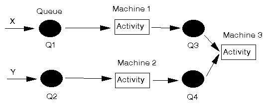
Well if Q4 is large then this is EITHER because Machine 3 is fully utilised OR because there are no X parts to be assembled together with Y parts. Here we know from the server utilisation figures that Machine 3 is not fully utilised, so the problem is an absence of X parts in Q3.
This absence could be caused by a bottleneck at Machine 1, but we know this is not so because utilisation statistics (and indeed queue statistics for Q1) tell us so. Hence we FINALLY have an answer as to why adding an extra Machine 4, which was the previous bottleneck, has not doubled production. Simply put not enough X parts are entering the system to enable production to be doubled.
Whilst (hopefully) I have explained the reasoning logically enough for you now to be clear about why the effect of adding an extra Machine 4 was not as we might have expected reflect for yourself on whether, when we first posed the question above as to the effect of adding an extra Machine 4, you successfully predicted the effect or not.