OR-Notes are a series of introductory notes on topics that fall under the broad heading of the field of operations research (OR). They were originally used by me in an introductory OR course I give at Imperial College. They are now available for use by any students and teachers interested in OR subject to the following conditions.
A full list of the topics available in OR-Notes can be found here.
Queuing theory deals with problems which involve queuing (or waiting). Typical examples might be:
As we know queues are a common every-day experience. Queues form because resources are limited. In fact it makes economic sense to have queues. For example how many supermarket tills you would need to avoid queuing? How many buses or trains would be needed if queues were to be avoided/eliminated?
In designing queueing systems we need to aim for a balance between service to customers (short queues implying many servers) and economic considerations (not too many servers).
In essence all queuing systems can be broken down into individual sub-systems consisting of entities queuing for some activity (as shown below).
Typically we can talk of this individual sub-system as dealing with customers queuing for service. To analyse this sub-system we need information relating to:
The simplest arrival process is one where we have completely regular arrivals (i.e. the same constant time interval between successive arrivals). A Poisson stream of arrivals corresponds to arrivals at random. In a Poisson stream successive customers arrive after intervals which independently are exponentially distributed. The Poisson stream is important as it is a convenient mathematical model of many real life queuing systems and is described by a single parameter - the average arrival rate. Other important arrival processes are scheduled arrivals; batch arrivals; and time dependent arrival rates (i.e. the arrival rate varies according to the time of day).
Assuming that the service times for customers are independent and do not depend upon the arrival process is common. Another common assumption about service times is that they are exponentially distributed.
Changing the queue discipline (the rule by which we select the next customer to be served) can often reduce congestion. Often the queue discipline "choose the customer with the lowest service time" results in the smallest value for the time (on average) a customer spends queuing.
Note here that integral to queuing situations is the idea of uncertainty in, for example, interarrival times and service times. This means that probability and statistics are needed to analyse queuing situations.
In terms of the analysis of queuing situations the types of questions in which we are interested are typically concerned with measures of system performance and might include:
These are questions that need to be answered so that management can evaluate alternatives in an attempt to control/improve the situation. Some of the problems that are often investigated in practice are:
In order to get answers to the above questions there are two basic approaches:
The reason for there being two approaches (instead of just one) is that analytic methods are only available for relatively simple queuing systems. Complex queuing systems are almost always analysed using simulation (more technically known as discrete-event simulation).
The simple queueing systems that can be tackled via queueing theory essentially:
The first queueing theory problem was considered by Erlang in 1908 who looked at how large a telephone exchange needed to be in order to keep to a reasonable value the number of telephone calls not connected because the exchange was busy (lost calls). Within ten years he had developed a (complex) formula to solve the problem.
Additional queueing theory information can be found here and here
It is common to use to use the symbols:
There is a standard notation system to classify queueing systems as A/B/C/D/E, where:
Common options for A and B are:
If D and E are not specified then it is assumed that they are infinite.
For example the M/M/1 queueing system, the simplest queueing system, has a Poisson arrival distribution, an exponential service time distribution and a single channel (one server).
Note here that in using this notation it is always assumed that there is just a single queue (waiting line) and customers move from this single queue to the servers.
Suppose we have a single server in a shop and customers arrive in the shop with a Poisson arrival distribution at a mean rate of lamda=0.5 customers per minute, i.e. on average one customer appears every 1/lamda = 1/0.5 = 2 minutes. This implies that the interarrival times have an exponential distribution with an average interarrival time of 2 minutes. The server has an exponential service time distribution with a mean service rate of 4 customers per minute, i.e. the service rate µ=4 customers per minute. As we have a Poisson arrival rate/exponential service time/single server we have a M/M/1 queue in terms of the standard notation.
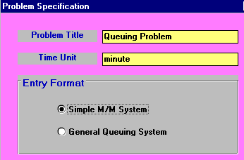
We can analyse this queueing situation using the package. The input is shown below:

with the output being:
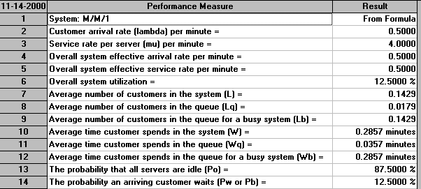
The first line of the output says that the results are from a formula. For this very simple queueing system there are exact formulae that give the statistics above under the assumption that the system has reached a steady state - that is that the system has been running long enough so as to settle down into some kind of equilibrium position.
Naturally real-life systems hardly ever reach a steady state. Simply put life is not like that. However despite this simple queueing formulae can give us some insight into how a system might behave very quickly. The package took a fraction of a second to produce the output seen above.
One factor that is of note is traffic intensity = (arrival rate)/(departure rate) where arrival rate = number of arrivals per unit time and departure rate = number of departures per unit time. Traffic intensity is a measure of the congestion of the system. If it is near to zero there is very little queuing and in general as the traffic intensity increases (to near 1 or even greater than 1) the amount of queuing increases. For the system we have considered above the arrival rate is 0.5 and the departure rate is 4 so the traffic intensity is 0.5/4 = 0.125
Consider the situation we had above - which would you prefer:
The simple answer is that we can analyse this using the package. For the first situation one server working twice as fast corresponds to a service rate µ=8 customers per minute. The output for this situation is shown below.

For two servers working at the original rate the output is as below. Note here that this situation is a M/M/2 queueing system. Note too that the package assumes that these two servers are fed from a single queue (rather than each having their own individual queue).


Compare the two outputs above - which option do you prefer?
Of the figures in the outputs above some are identical. Extracting key figures which are different we have:
                                    One server twice as fast   Two servers, original rate
Average time in the system                  0.1333                     0.2510
(waiting and being served)
Average time in the queue                   0.0083                     0.0010
Probability of having to wait for service   6.25%                      0.7353%
It can be seen that with one server working twice as fast customers spend less time in the system on average, but have to wait longer for service and also have a higher probability of having to wait for service.
Below we have extended the example we had before where now we have multiplied the customer arrival rate by a factor of six (i.e. customers arrive 6 times as fast as before). We have also entered a queue capacity (waiting space) of 2 - i.e. if all servers are occupied and 2 customers are waiting when a new customer appears then they go away - this is known as balking.
We have also added cost information relating to the server and customers:
The package input is shown below:
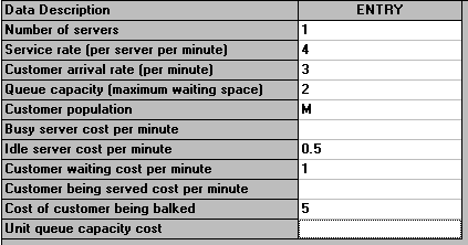
with the output being:

Note, as the above output indicates, that this is an M/M/1/3 system since we have 1 server and the maximum number of customers that can be in the system (either being served or waiting) is 3 (one being served, two waiting).
The key here is that as we have entered cost data we have a figure for the total cost of operating this system, 3.0114 per minute (in the steady state).
Suppose now we were to have two servers instead of one - would the cost be less or more? The simple answer is that the package can tell us, as below. Note that this is an M/M/2/4 queueing system as we have two servers and a total number of customers in the system of 4 (2 being served, 2 waiting in the queue for service). Note too that the package assumes that these two servers are fed from a single queue (rather than each having their own individual queue).
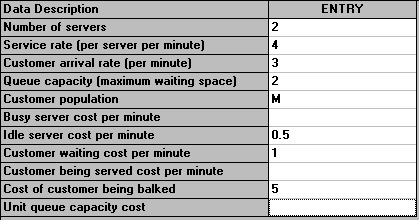
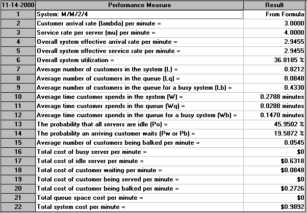
So we can see that there is a considerable cost saving per minute in having two servers instead of one.
In fact the package can automatically perform an analysis for us of how total cost varies with the number of servers. This can be seen below.
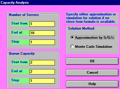
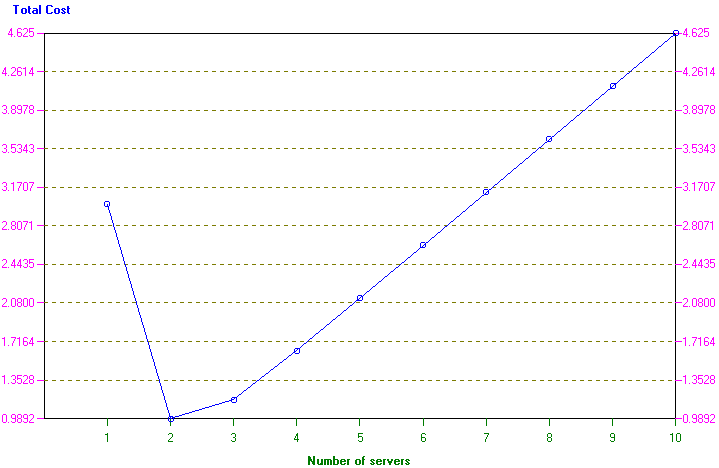
The screen below shows the possible input parameters to the package in the case of a general queueing model (i.e. not a M/M/r system).

Here we have a number of possible choices for the service time distribution and the interarrival time distribution. In fact the package recognises some 15 different distributions! Other items mentioned above are:
As an indication of the analysis that can be done an example problem is shown below:
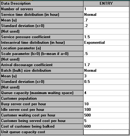
Solving the problem we get:
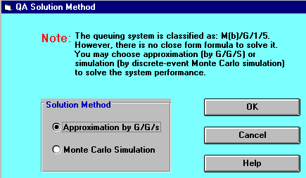
This screen indicates that no formulae exist to evaluate the situation we have set up. We can try to evaluate this situation using an approximation formula, or by Monte Carlo Simulation. If we choose to adopt the approximation approach we get:
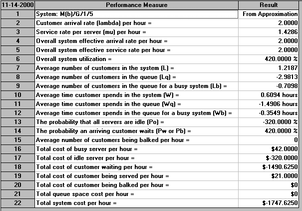
The difficulty is that these approximation results are plainly nonsense (i.e. not a good approximation). For example the average number of customers in the queue is -2.9813, the probability that all servers are idle is -320%, etc. Whilst for this particular case it is obvious that approximation (or perhaps the package) is not working, for other problems it may not be readily apparent that approximation does not work.
If we adopt the Monte Carlo Simulation approach then we have the screen below.
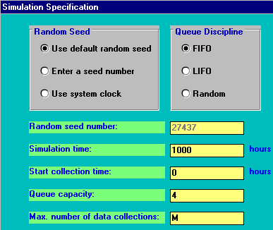
What will happen here is that the computer will construct a model of the system we have specified and internally generate customer arrivals, service times, etc and collect statistics on how the system performs. As specified above it will do this for 1000 time units (hours in this case). The phrase "Monte Carlo" derives from the well-known gambling city on the Mediterranean in Monaco. Just as in roulette we get random numbers produced by a roulette wheel when it is spun, so in Monte Carlo simulation we make use of random numbers generated by a computer.
The results are shown below:

These results seem much more reasonable than the results obtained the approximation.
However one factor to take into consideration is the simulation time we specified - here 1000 hours. In order to collect more accurate information on the behaviour of the system we might wish to simulate for longer. The results for simulating both 10 and 100 times as long are shown below.

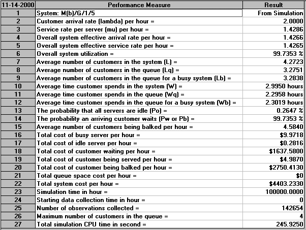
Clearly the longer we simulate, the more confidence we may have in the statistics/probabilities obtained.
As before we can investigate how the system might behave with more servers. Simulating for 1000 hours (to reduce the overall elapsed time required) and looking at just the total system cost per hour (item 22 in the above outputs) we have the following:
Number of servers   Total system cost
       1                  4452
       2                  3314
       3                  2221
       4                  1614
       5                  1257
       6                   992
       7                   832
       8                   754
       9                   718
      10                   772
      11                   833
      12                   902
Hence here the number of servers associated with the minimum total system cost is 9