OR-Notes

J E Beasley

OR-Notes are a series of introductory notes on topics that fall under the broad heading of the field of operations research (OR). They were originally used by me in an introductory OR course I give at Imperial College. They are now available for use by any students and teachers interested in OR subject to the following conditions.

A full list of the topics available in OR-Notes can be found here.

Network analysis - uncertain completion times

One important extension to the basic network analysis technique relates to uncertain activity completion times. In this extension to the basic method we give, for each activity, not a single completion time but three times:

• optimistic time (t₁) - the completion time if all goes well
• most likely (modal) time (t₂) - the completion time we would expect under normal conditions
• pessimistic time (t₃) - the completion time if things go badly.

This use of three time estimates is the PERT technique. Note here that these three time estimates do not imply that, when the activity is performed, its completion time will be one of three choices - optimistic, most likely or pessimistic. Instead these three numbers are used to produce an underlying probability distribution of completion times such that all times are possible (with an associated probability).

These three times are combined into a single figure, the expected activity completion time, given by (t₁ + 4t₂ + t₃)/6 and this figure is used as the activity completion time when carrying out the calculations presented before to find the project completion time and the critical activities.

Note here that this weighting of optimistic:most likely:pessimistic of 1/6:4/6:1/6 is essentially fixed and cannot be altered (as the underlying theory depends on these weights).

In addition, through the use of the beta and normal probability distributions, we can get an idea of how this project completion time might vary (remember we no longer know the individual activity completion times with certainty).

Essentially we can find answers to questions like:

• What is the probability that the project will take longer than...?
• What is the probability that the project will be finished by...?

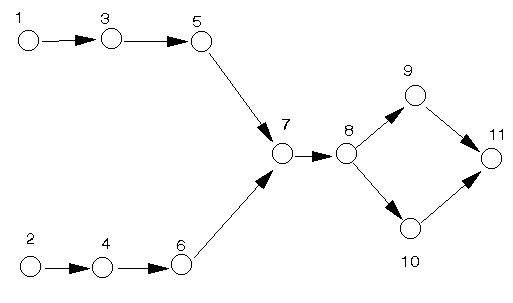
To illustrate this consider the package input shown below where, for the activity on node network we had before, (also reproduced below) we now have an optimistic time equal to one-half the most likely time and a pessimistic time equal to twice the most likely time.

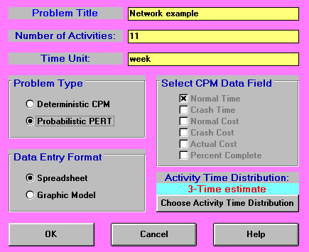
In the input shown above we have specified a 3-time estimate for the activity time distribution. The package allows us to alter this (to a considerable extent), but we must be sure that our implicit assumption as to which activity time distribution applies is justified.

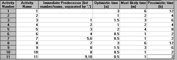
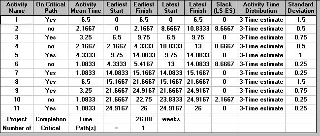
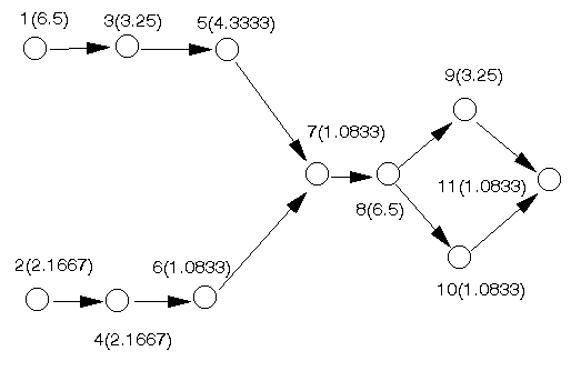
The output from the package for this example is shown below. Note here that one of the columns in that figure corresponds to the expected (mean) activity completion time of (t₁ + 4t₂ + t₃)/6. All of the earliest/latest start/finish time calculations are performed with respect to this expected (mean) time. You can see from below that we expect to finish this project in 26 weeks.

The network, from which we calculate the above figures, together with the expected times for each activity, is shown below.

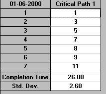
In the above package output the final column is labelled Standard Deviation. As we have a statistical distribution for the completion time of each activity (as represented by the optimistic, most likely and pessimistic times) we also have an underlying statistical variation in the completion time - as represented by the standard deviation. This standard deviation is calculated as (t₃ - t₁)/6. The critical path is shown below.

Probability analysis

Below we show the probability analysis obtainable from the package where, for any project completion time, we have an estimate of the probability of finishing the project within that time. In the example below we have chosen to estimate the probability of completing the project within 27 weeks.

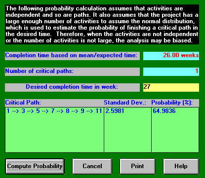
It can be seen that although the expected completion time is 26 weeks the probability of completing within any time up to and including 27 weeks is 64.9836%. We can also carry out this probability calculation for a number of other completion times, as below for 25 weeks and 26 weeks.

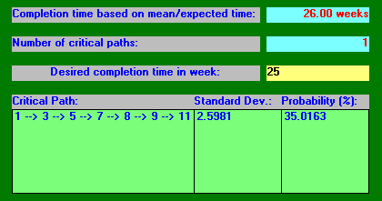
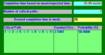
Note especially here how the probability of completing within the expected completion time of 26 weeks is only 50%.

Using this probability analysis it is possible to construct the graph shown below where, for a range of possible project completion times, we have plotted the probability that the project has been completed by that time.

Note here that the curve shown above is not fixed - we may be able to change its shape by refining the time estimates (optimistic, most likely, pessimistic) we used which led to the curve, i.e. to reduce the uncertainty associated with each activity, and hence reduce the uncertainty associated with the completion of the entire project.

It is clear that in order for the final probability curve, such as that shown above, to be accurate our time estimates must also be accurate. One approach that can be followed is to systematically review the time estimates associated with the critical activities, since it is the critical activities that are used in establishing the above probability curve (as will become clearer below). However note that any non-critical activities whose completion times have been underestimated are also important (non-critical activities whose completion times have been over-estimated are obviously of lesser importance).

One approach that can be followed in examining critical activities with respect to uncertainty is to see if the activity can be subdivided into sub-activities. The advantage of this is that it may be that some of these sub-activities have low uncertainty with respect to their completion times (i.e. we are fairly sure as to how long they may take). For example suppose we were to split activity 1 into 2 sub-activities (1a and 1b) as follows:

• activity 1a optimistic time 2, most likely time 3, pessimistic time 4 - hence an expected time of 2(1/6) + 3(4/6) + 4(1/6) = 3 and a standard deviation of (4-2)/6 = 0.3333
• activity 1b optimistic time 1, most likely time 3, pessimistic time 8 - hence an expected time of 1(1/6) + 3(4/6) + 8(1/6) = 3.5 and a standard deviation of (8-1)/6 = 1.1667

Then by elementary statistical theory these sub-activities together have an expected time of 3 + 3.5 = 6.5 (the original expected time for activity 1) and a standard deviation equal to [(0.3333)² + (1.1667)²]^0.5 = 1.2134, lower then the previous standard deviation of 1.5. A lower standard deviation implies more certainty so, by splitting activity 1, we are actually more certain about how long it will take. This reduction in uncertainty is plainly of benefit.

Manual probability calculation

The probability calculation carried out above by computer can also be done without the aid of a computer. To calculate the probability that the project will be completed by time T we first:

• calculate the expected (mean) completion time for each activity
• work out the overall project completion time and the critical activities using the single figure of expected (mean) time for each activity, as we have seen how to do previously
• list the critical paths in the network

Then for each critical path in turn, which are all of equal mean completion time C, we calculate the sum of the variances of each activity on the critical path. Variance (as you may recall from any statistics background you have) is the square of standard deviation. Let this sum be V. Calculate z=(T-C)/V^0.5. Then the probability that each critical path will be completed by time T is given by the probability of observing a value from the standard normal distribution N(0,1) with value z or less. Such values are given below.

Then take these probabilities for each of the critical paths and multiply them together. This product gives the probability that the entire project will be completed by time T.

To illustrate this let us take T=27 and the network we considered above. We already have the critical path of 1-3-5-7-8-9-11 calculated using the expected (mean) completion times, although we could have done this calculation without a computer if necessary. Note here that for this problem there is only one critical path.

Hence V = (1.5)² + (0.75)² + 1² + (0.25)² + (1.5)² + (0.75)² + (0.25)² = 6.75

and the sd is hence (6.75)^0.5 = 2.5981, equal to the value given by the computer before.

We know C=26 (the expected completion time for the critical path) so z=(T-C)/V^0.5 = (27-26)/(6.75)^0.5 = 0.38

Now the standard statistical table tabulating, for values of z, the associated probabilities is shown below. To use this table for z=0.38 first find the row containing 0.3 and then look across to the 0.08 column. The associated probability value can then be read directly and is in this case 0.648.

Hence the probability of observing a value from the standard normal distribution N(0,1) with value 0.38 or less is 0.648 = 64.8%. Hence as we have only one critical path the probability that the entire project will be completed within 27 weeks is 64.8%.

Compared to the value of 64.9836% given above it seems that we have a discrepancy. In fact this arises simply because we have truncated to two decimal places in computing 0.38 from (27-26)/(6.75)^0.5. To three decimal places (27-26)/(6.75)^0.5 is 0.385 and so a more accurate probability is given by averaging the entries in the table below for 0.38 and 0.39 i.e. (0.648+0.652)/2 = 0.65 = 65% which compares well with the value of 64.9836% given above.

N(0,1) values

As a further illustration for T=25 we have that z=(T-C)/V^0.5 = (25-26)/(6.75)^0.5 = -0.385 (since C and V are as before). To find the value in the table above associated with a negative z value simply take 1- the value associated with the positive z value. Here we already know that the value associated with the positive z value is 0.65 so 1-0.65 =0.35 = 35%. Hence the probability of completing the project within 25 weeks is 35 %. This compares well with the figure given above by the package of 35.0163%.

For those of you with a more statistical background the above probability calculation makes a number of assumptions. e.g. see

These assumptions are essentially that:

• the normal distribution can be applied (e.g. by invoking the Central Limit Theorem); and that
• the critical paths are independent (have no activities in common).

This second assumption is used when we multiply together the probabilities of each critical path being completed by a certain time in order to calculate the probability of the overall project being completed by a certain time.

Hence one needs to be aware that the probability figures calculated may be inaccurate.

Simulation

The above probability analysis was done using statistical probability theory. An alternative approach to estimating the probability of the project being completed by a certain time T is to use discrete-event simulation. In this approach we, for a number of trials (simulated observations):

• sample a completion time for each activity based upon its underlying statistical completion time distribution
• calculate how long the project will take using these sampled times

and then estimate the probability of completing the project by T using (number of trials in which project was completed by T)/(total number of trials).

This is shown below using the package for T=27 weeks and 1000 trials.

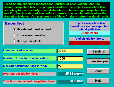
You can see above how the simulated probability of 66.3% is relatively close to the previous calculated probability of 64.9836%. If we increase the number of trials to 10000 we might expect to get closer to this previously calculated figure. In fact we get the result below, moving further away.

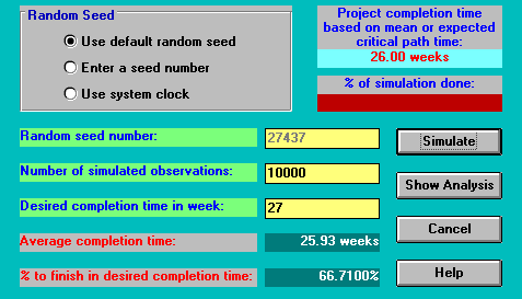
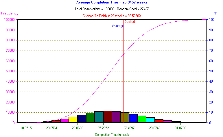
Increasing the number of trials further to 100000 results in:

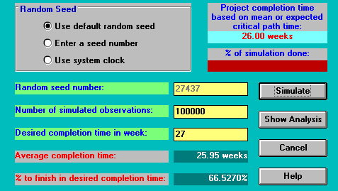
It is clear therefore that we are not achieving any convergence between the simulated probability and the previously calculated probability. When a discrepancy such as this arises the usual causes are:

• the assumptions mentioned above underlying the probability calculation are not true
• the random number generator used to sample a completion time for each activity is not a good one, i.e. that it does not produce numbers which can really be said to be random
• coding error

With a small network like the one we have considered the most likely reason for the discrepancy in this case is that the assumptions mentioned above underlying the probability calculation are not true, probably because there are not sufficient activities for the Normal distribution to apply via the Central Limit Theorem.

You should be clear therefore that although the probability calculation gives you a quick, and seemingly accurate, figure it is wise to check this figure using simulation (which is slow, but may reveal that the assumptions underlying the probability calculation were not true).

Note too here that the simulation analysis, as well as giving you a probability of finishing within a desired completion time can also produce a graphic representation of the project completion time distribution. This is shown below for the simulation associated with 100000 trials given above.

This point about checking the probability figure is especially important for either end of the probability curve, far from the expected project completion time (26 weeks in this case). For example the probability calculated via the package for completing within 33 weeks is 99.6465%. Performing the simulation we get:

• 1000 trials, probability 99.7%
• 10000 trails, probability 99.61%
• 100000 trails, probability 99.665%

So in this case we have a fairly good correspondence.