OR-Notes are a series of introductory notes on topics that fall under the broad heading of the field of operations research (OR). They were originally used by me in an introductory OR course I give at Imperial College. They are now available for use by any students and teachers interested in OR subject to the following conditions.
A full list of the topics available in OR-Notes can be found here.
A company manufactures four variants of the same product and in the final part of the manufacturing process there are assembly, polishing and packing operations. For each variant the time required for these operations is shown below (in minutes) as is the profit per unit sold.
                Assembly      Polish    Pack        Profit (£)
Variant 1       2             3         2           1.50
        2       4             2         3           2.50
        3       3             3         2           3.00
        4       7             4         5           4.50
Let:
xi be the number of units of variant i (i=1,2,3,4) made per year
Tass be the number of minutes used in assembly per year
Tpol be the number of minutes used in polishing per year
Tpac be the number of minutes used in packing per year
where xi >= 0 i=1,2,3,4 and Tass, Tpol, Tpac >= 0
(a) operation time definition
Tass = 2x1 + 4x2 + 3x3 +
7x4 (assembly)
Tpol = 3x1 + 2x2 + 3x3 + 4x4
(polish)
Tpac = 2x1 + 3x2 + 2x3 + 5x4
(pack)
(b) operation time limits
The operation time limits depend upon the situation being considered. In the first situation, where the maximum time that can be spent on each operation is specified, we simply have:
Tass <= 100000 (assembly)
Tpol <= 50000 (polish)
Tpac <= 60000 (pack)
In the second situation, where the only limitation is on the total time spent on all operations, we simply have:
Tass + Tpol + Tpac <= 210000 (total time)
Presumably to maximise profit - hence we have
maximise 1.5x1 + 2.5x2 + 3.0x3 + 4.5x4
Solution - using Solver
Below we solve this LP with the Solver add-in that comes with Microsoft Excel.
If you click here you will be able to download an Excel spreadsheet called lp.xls that already has the LP we are considering set up.
Take this spreadsheet and look at Sheet A. You should see the problem we considered above set out as:

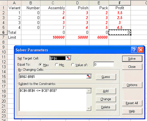
Here the values in cells B2 to B5 are how much of each variant we choose to make - here set to zero. Cells C6 to E6 give the total assembly/polishing and packing time used and cell F6 the total profit associated with the amount we choose to produce.
To use Solver in Excel do Tools and then Solver. In the version of Excel I am using (different versions of Excel have slightly different Solver formats) you will get the Solver model as below:

Here our target cell is F6 (ignore the use of $ signs here - that is a technical Excel issue if you want to go into it in greater detail) which we wish to maximise. We can change cells B2 to B5 - i.e. the amount of each variant we produce subject to the constraint that C6 to E6 - the total amount of assembly/polishing/packing used cannot exceed the limits given in C7 to E7.
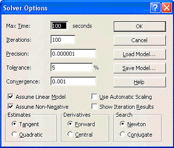
In order to tell Solver we are dealing with a linear program click on Options in the Solver box and you will see:

where both the 'Assume Linear Model' and 'Assume Non-Negative' boxes are ticked - indicating we are dealing with a linear model with non-negative variables.
Solving via Solver the solution is:

We can see that the optimal solution to the LP has value 58000 (£) and that Tass=82000, Tpol=50000, Tpac=60000, X1=0, X2=16000, X3=6000 and X4=0.
This implies that we only produce variants 2 and 3 (a somewhat surprising result in that we are producing none of variant 4 which had the highest profit per unit produced).
Referring back to the physical situation we can see that at the LP optimal we have 18,000 minutes of assembly time that is not used (Tass=82000 compared with a maximum time of 100000) but that all of the polishing and packing time is used.
For the second situation given in the question, where the only limitation is on the total time spent on all operations examine Sheet B in spreadsheet lp.xls
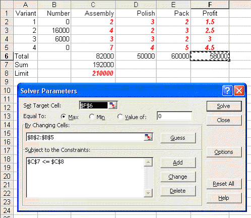
Invoking Solver in that sheet you will see:

where cell C7 is the total amount of processing time used and the only constraint in Solver relates to that cell not exceeding the limit of 210000 shown in cell C8. Note here that if you check Options in Solver here you will see that both the 'Assume Linear Model' and 'Assume Non-Negative' boxes are ticked.
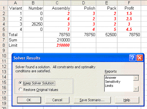
Solving we get:

We can see that the optimal solution to the LP has value 78750 (£) and that Tass=78750, Tpol=78750, Tpac=52500, X1=0, X2=0, X3=26250 and X4=0.
This implies that we only produce variant 3.
Note here how much higher the associated profit is than before (£78750 compared with £58000, an increase of 36%!). This indicates that, however the allocation given before of 100,000; 50,000 and 60,000 minutes for assembly, polishing and packing respectively was arrived at it was a bad decision!
Problem sensitivity refers to how the solution changes as the data changes. Two issues are important here:
We deal with each of these in turn.
Robustness
Plainly, in the real world, data is never completely accurate and so we would like some confidence that any proposed course of action is relatively insensitive (robust) with respect to data inaccuracies. For example, for the production planning problem dealt with before, how sensitive is the optimal solution with respect to slight variations in any particular data item.
For example consider the packing time consumed by variant 3. It is currently set to exactly 2 minutes, i.e. 2.0000000. But suppose it is really 2.1, what is the effect of this on what we are proposing to do?
What is important here is what you might call "the shape of the strategy" rather than the specific numeric values. Look at the solution of value 58000 we had before. The shape of the strategy there was "none of variant 1 or 4, lots of variant 2 and a reasonable amount of variant 3". What we would like is that, when we resolve with the figure of 2 for packing time consumed by variant 3 replaced by 2.1, this general shape remains the same. What might concern us is if we get a very different shape (e.g. variants 1 and 4 only).
If the general shape of the strategy remains essentially the same under (small) data changes we say that the strategy is robust.
If we take Sheet A again, change the figure of 2 for packing time consumed by variant 3 to 2.1 and resolve we get:

This indicates that for this data change the strategy is robust.
Planning
With regard to planning we may be interested in seeing how the solution changes as the data changes (e.g. over time). For example for the production planning problem dealt with above (where the solution was of value 58000 involving production of variants 2 and 3) how would increasing the profit per unit on variant 4 (e.g. by 10 per cent to 4.95 by raising the price) impact upon the optimal solution.
Again taking Sheet A, making the appropriate change and resolving, we get:

indicating that if we were able to increase the profit per unit on variant 4 by 10 per cent to 4.95 it would be profitable to make that variant in the quantities shown above.
There is one thing to note here - namely that we have a fractional solution X3=1428.571 and X4=11428.57. Recall that we have a linear program - for which a defining characteristic is that the variables are allowed to take fractional values. Up to now for this production planning problem we had not seen any fractional values when we solved numerically - here we do. Of course in reality, given that the numbers are large there is no practical significance to these fractions and we can equally well regard the solution as being a conventional integer (non-fractional) solution such as X3=1429 and X4=11429.
Approach
In fact the approach taken both for robustness and planning issues is identical, and is often referred to as sensitivity analysis.
Given the LP package it is a simple matter to change the data and resolve to see how the solution changes (if at all) as certain key data items change.
In fact, as a by-product of using the simplex algorithm, we automatically get sensitivity information.However, interpreting simplex sensitivity information is somewhat complicated and so, for the purposes of this course, I prefer to approach sensitivity via resolving the LP. Those interested in interpreting the sensitivity information automatically produced by the simplex algorithm can find some information here.
Some other linear programming solution examples can be found here.