OR-Notes are a series of introductory notes on topics that fall under the broad heading of the field of operations research (OR). They were originally used by me in an introductory OR course I give at Imperial College. They are now available for use by any students and teachers interested in OR subject to the following conditions.
A full list of the topics available in OR-Notes can be found here.
Recall the production planning problem concerned with four variants of the same product which we formulated before as an LP. To remind you of it we repeat below the problem and our formulation of it.
A company manufactures four variants of the same product and in the final part of the manufacturing process there are assembly, polishing and packing operations. For each variant the time required for these operations is shown below (in minutes) as is the profit per unit sold.
                Assembly      Polish    Pack        Profit (£)
Variant 1       2             3         2           1.50
        2       4             2         3           2.50
        3       3             3         2           3.00
        4       7             4         5           4.50
Let:
xi be the number of units of variant i (i=1,2,3,4) made per year
Tass be the number of minutes used in assembly per year
Tpol be the number of minutes used in polishing per year
Tpac be the number of minutes used in packing per year
where xi >= 0 i=1,2,3,4 and Tass, Tpol, Tpac >= 0
(a) operation time definition
Tass = 2x1 + 4x2 + 3x3 +
7x4 (assembly)
Tpol = 3x1 + 2x2 + 3x3 + 4x4
(polish)
Tpac = 2x1 + 3x2 + 2x3 + 5x4
(pack)
(b) operation time limits
The operation time limits depend upon the situation being considered. In the first situation, where the maximum time that can be spent on each operation is specified, we simply have:
Tass <= 100000 (assembly)
Tpol <= 50000 (polish)
Tpac <= 60000 (pack)
In the second situation, where the only limitation is on the total time spent on all operations, we simply have:
Tass + Tpol + Tpac <= 210000 (total time)
Presumably to maximise profit - hence we have
maximise 1.5x1 + 2.5x2 + 3.0x3 + 4.5x4
which gives us the complete formulation of the problem.
Solution - using Solver
Below we solve this LP with the Solver add-in that comes with Microsoft Excel.
If you click here you will be able to download an Excel spreadsheet called lp.xls that already has the LP we are considering set up.
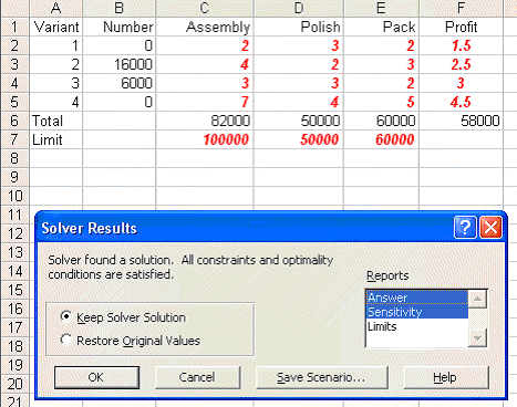
Look at Sheet A in lp.xls and to use Solver do Tools and then Solver. In the version of Excel I am using (different versions of Excel have slightly different Solver formats) you will get the Solver model as below:

but where now we have highlighted (clicked on) two of the Reports available - Answer and Sensitivity. Click OK and you will find that two new sheets have been added to the spreadsheet - an Answer Report and a Sensitivity Report.
As these reports are indicative of the information that is commonly available when we solve a LP via a computer we shall deal with each of them in turn.
Answer Report
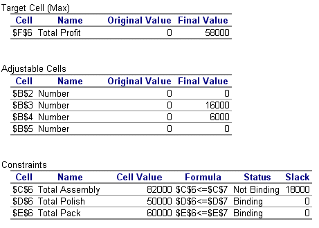
The answer report can be seen below:

This is the most self-explanatory report.
We can see that the optimal solution to the LP has value 58000 (£) and that Tass=82000, Tpol=50000, Tpac=60000, X1=0, X2=16000, X3=6000 and X4=0.
Note that we had three constraints for total assembly, total polishing and total packing time in our LP. The assembly time constraint is declared to be 'Not Binding' whilst the other two constraints are declared to be 'Binding'. Constraints with a 'Slack' value of zero are said to be tight or binding in that they are satisfied with equality at the LP optimal. Constraints which are not tight are called loose or not binding.
Sensitivity Report
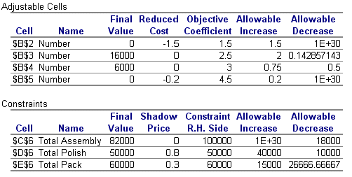
The sensitivity report can be seen below:

This sensitivity report provides us with information relating to:
We deal with each of these in turn, and note here that the analysis presented below ONLY applies for a single change, if two or more things change then we effectively need to resolve the LP.
Changing the objective function coefficient for a variable
To illustrate this suppose we vary the coefficient of X2 in the objective function. How will the LP optimal solution change?
Currently X1=0, X2=16000, X3=6000 and X4=0. The current solution value for X2 of 16000 is in cell B3 and the current objective function coefficient for X2 is 2.5. The Allowable Increase/Decrease columns tell us that, provided the coefficient of X2 in the objective function lies between 2.5+2 = 4.5 and 2.5 - 0.142857143 = 2.3571 (to four decimal places), the values of the variables in the optimal LP solution will remain unchanged. Note though that the actual optimal solution value will change as the objective function coefficient of X2 is changing.
In terms of the original problem we are effectively saying that the decision to produce 16000 of variant 2 and 6000 of variant 3 remains optimal even if the profit per unit on variant 2 is not actually 2.5 (but lies in the range 2.3571 to 4.50). Similar conclusions can be drawn about X1, X3 and X4.
Forcing a variable which is currently zero to be non-zero
For the variables, the Reduced Cost column gives us, for each variable which is currently zero (X1 and X4), an estimate of how much the objective function will change if we make (force) that variable to be non-zero. Note here that the value in the Reduced Cost column for a variable is often called the 'opportunity cost' for the variable.
Hence we have the table
Variable                             X1      X4
Reduced Cost (opportunity cost)      1.5     0.2
New value (= or >=)                  X1=A    X4=B
                                  or X1>=A   X4>=B
Estimated objective function change  1.5A    0.2B
where we ignore the sign of the reduced cost when constructing the above table. The objective function will always get worse (go down if we have a maximisation problem, go up if we have a minimisation problem) by at least this estimate. The larger A or B are the more inaccurate this estimate is of the exact change that would occur if we were to resolve the LP with the corresponding constraint for the new value of X1 or X4 added.
Note here than an alternative (and equally valid) interpretation of the reduced cost is the amount by which the objective function coefficient for a variable needs to change before that variable will become non-zero.
Hence for variable X1 the objective function needs to change by 1.5 (increase since we are maximising) before that variable becomes non-zero. In other words, referring back to our original situation, the profit per unit on variant 1 would need to increase by 1.5 before it would be profitable to produce any of variant 1. Similarly the profit per unit on variant 4 would need to increase by 0.2 before it would be profitable to produce any of variant 4.
Changing the right-hand side of a constraint
For each constraint the column headed Shadow Price tells us exactly how much the objective function will change if we change the right-hand side of the corresponding constraint within the limits given in the Allowable Increase/Decrease columns
Hence we can form the table
Constraint                                  Assembly    Polish    Pack
Opportunity (Reduced) Cost (ignore sign)    0           0.80      0.30
Change in right-hand side                   a           b         c
Objective function change                   0           0.80b     0.30c
Lower limit for right-hand side             82000       40000     33333.34
Current value for right-hand side           100000      50000     60000
Upper limit for right-hand side             -           90000     75000
For example for the polish constraint, provided the right-hand side of that constraint remains between 50000 + 40000 =90000 and 50000 - 10000 = 40000 the objective function change will be exactly 0.80[change in right-hand side from 50000].
The direction of the change in the objective function (up or down) depends upon the direction of the change in the right-hand side of the constraint and the nature of the objective (maximise or minimise).
To decide whether the objective function will go up or down use:
Hence
The value in the column headed Shadow Price for a constraint is often called the 'marginal value' or 'dual value' for that constraint.
Note that, as would seem logical, if the constraint is loose the shadow price is zero (as if the constraint is loose a small change in the right-hand side cannot alter the optimal solution).
Note here that, as mentioned above, the analysis given above relating to:
is only valid for a single change. If two (or more) changes are made the situation becomes more complex and it becomes advisable to resolve the LP.