OR-Notes are a series of introductory notes on topics that fall under the broad heading of the field of operations research (OR). They were originally used by me in an introductory OR course I give at Imperial College. They are now available for use by any students and teachers interested in OR subject to the following conditions.
A full list of the topics available in OR-Notes can be found here.
When we dealt with network analysis previously we were concerned with just a single project, where the implicit assumption was that we had already decided to do the project. Suppose now that we are considering four possible projects, which each run for 3 years and have the following characteristics:
                         Capital requirements (£m)
Project   Return (£m)    Year   1     2     3
1         0.2                   0.5   0.3   0.2
2         0.3                   1.0   0.8   0.2
3         0.5                   1.5   1.5   0.3
4         0.1                   0.1   0.4   0.1
Available capital (£m)          3.1   2.5   0.4
We have a decision problem here: Which projects would you choose in order to maximise the total return?
Note here that, from the project management viewpoint, the focus has moved from the tactical consideration of how to organise the project which we considered previously under network analysis (cost/time tradeoff, uncertain activity completion times, resource restrictions, etc) to a more strategic viewpoint.
This problem can be formulated and solved as an integer programming problem. Such problems arise when (as we shall see below) the variables in the formulation of the problem must take integer (discrete) values. Problems in which this is the case are called integer programs (IP's) and the subject of solving such programs is called integer programming (also referred to by the initials IP).
IP's occur frequently because many decisions are essentially discrete (such as yes/no, go/no-go) in that one (or more) options must be chosen from a finite set of alternatives.
Note here that problems in which some variables can take only integer values and some variables can take fractional values are called mixed-integer programs (MIP's).
Solution
In order to solve our project selection example we follow the same approach as we used for formulating LP's - namely:
We do this below and note here that the only significant change in formulating IP's as opposed to formulating LP's is in the definition of the variables.
Here we are trying to decide whether to undertake a project or not (a "go/no-go" decision). One "trick" in formulating IP's is to introduce variables which take the integer values 0 or 1 and represent binary decisions (e.g. do a project or not do a project) with typically:
Such variables are often called zero-one or binary variables
To define the variables we use the verbal description of
xj = 1 if we decide to do project j (j=1,...,4)
   = 0 otherwise, i.e. not do project j (j=1,...,4)
Note here that, by definition, the xj are integer variables which must take one of two possible values (zero or one).
The constraints relating to the availability of capital funds each year are
0.5x1 + 1.0x2 + 1.5x3 + 0.1x4
<= 3.1 (year 1)
0.3x1 + 0.8x2 + 1.5x3 + 0.4x4
<= 2.5 (year 2)
0.2x1 + 0.2x2 + 0.3x3 + 0.1x4
<= 0.4 (year 3)
To maximise the total return - hence we have
maximise 0.2x1 + 0.3x2 + 0.5x3 + 0.1x4
This gives us the complete IP which we write as
maximise 0.2x1 + 0.3x2 + 0.5x3 + 0.1x4
subject to
0.5x1 + 1.0x2 + 1.5x3 + 0.1x4
<= 3.1
0.3x1 + 0.8x2 + 1.5x3 + 0.4x4
<= 2.5
0.2x1 + 0.2x2 + 0.3x3 + 0.1x4
<= 0.4
xj = 0 or 1 j=1,...,4
Note:
Extensions to this basic problem include:
We shall consider these extensions below.
Extensions
Projects with different lengths are easily dealt with, just set their capital requirement in any year in which the project does not exist (i.e. has not started or has already ended) to zero. For example if project 1 only runs for 2 years (instead of 3 years) and hence finishes in year 2 then the capital requirement constraint for year 3 becomes:
0x1 + 0.2x2 + 0.3x3 + 0.1x4 <= 0.4
Projects with different start/end dates are dealt with in a similar manner as projects of different lengths, just set their capital requirements in any year in which they do not exist (i.e. they have not started or have already ended) to zero. For example if project 1 starts and ends in year 2; project 2 starts in year 2 and project 4 ends in year 2 then the capital requirement constraints become:
0x1 + 0x2 + 1.5x3 + 0.1x4
<= 3.1 (year 1)
0.3x1 + 0.8x2 + 1.5x3 + 0.4x4
<= 2.5 (year 2)
0x1 + 0.2x2 + 0.3x3 + 0x4 <=
0.4 (year 3)
If project 1 finishes in year 2, and all of the return from project 1 is available as capital in year 3 then this can be formulated by changing the capital requirement constraint for year 3 to:
0x1 + 0.2x2 + 0.3x3 + 0.1x4 <= 0.4 + 0.2x1
where note that we have 0x1 above as project 1 finishes in year 2 and hence has no capital requirement in year 3.
A question arises here in that if we put the return from a project into the capital for future years then should we be counting the return from the project in the objective function as well? One way to address this for project 1 here is to say that the return is split into two - one part y1 (say) that is counted as return taken in the objective and one part y2 (say) that is taken as return used for future capital in year 3. Then amending our formulation we have
y1 + y2 = 0.2x1
a balancing equality equation to correctly account for the return (since we may choose not to do project 1)
0x1 + 0.2x2 + 0.3x3 + 0.1x4 <= 0.4 + y2
to account for the capital added in year 3
maximise y1 + 0.3x2 + 0.5x3 + 0.1x4
to account for the return declared as profit.
Note here that y1 and y2 (both >=0) are continuous (fractional) variables so adding them in this way means that we have a mixed-integer program (MIP).
In this extension we have that a project gives a return at various stages over its lifetime, and this return can (perhaps) be used as capital to fund ongoing (or new) projects. To illustrate how this can be formulated consider project 1 which gives a total return of 0.2. Suppose now that this project gives a return of 0.15 at the end of year 2, and the remaining return of 0.05 in year 3. Suppose further that all of this "early" return can be used as available capital in year 3. Then the capital requirement constraint in year 3 becomes:
0.2x1 + 0.2x2 + 0.3x3 + 0.1x4 <= 0.4 + 0.15x1
In the example as currently formulated we have capital available in each year (3.1 in year 1, 2.5 in year 2 and 0.4 in year 3). In any particular year all of this capital may not be consumed by the projects that we choose to do. Suppose that we are allowed to carry forward (from year to year) 25% of any capital that is unused. To formulate this introduce linear (fractional) variables C12 and C23 (>=0) with C12 being the capital carried forward from year 1 to year 2 and C23 being the capital carried forward from year 2 to year 3. Then the constraints of the problem become:
0.5x1 + 1.0x2 + 1.5x3 + 0.1x4
<= 3.1 (year 1)
C12 = 0.25(3.1 - (0.5x1 + 1.0x2 + 1.5x3
+ 0.1x4))
0.3x1 + 0.8x2 + 1.5x3 + 0.4x4
<= 2.5 + C12 (year 2)
C23 = (2.5 + C12 - (0.3x1 + 0.8x2
+ 1.5x3 + 0.4x4))
0.2x1 + 0.2x2 + 0.3x3 + 0.1x4
<= 0.4 + C23 (year 3)
Suppose that projects 1 and 2 are mutually exclusive, i.e. we can choose to do one, or other, of these projects but not both. Then this can be formulated by adding to the problem the constraint:
x1 + x2 <= 1
This allows us to do neither of the projects (x1 = x2 = 0). If we wish to insist that we must do exactly one of these projects we can use
x1 + x2 = 1
Suppose that project 1 can start either in year 1, when it has the characteristics given above, or in year 2, when it has different characteristics - still the same return of 0.2 but a capital requirement of 0.9 in year 2 and 0.4 in year 3. Then this can be formulated by introducing a new zero-one variable y with y=1 representing choosing to do project 1 starting in year 2, y=0 representing not choosing to do project 1 starting in year 2. Then the capital requirement constraints for years 2 and 3 become:
0.3x1 + 0.8x2 + 1.5x3 + 0.4x4
+ 0.9y <= 2.5 (year 2)
0.2x1 + 0.2x2 + 0.3x3 + 0.1x4
+ 0.4y <= 0.4 (year 3)
We also need to add a constraint to prevent project 1 being started at more than one start time (i.e. project 1 starting in year 1 and project 1 starting in year 2 are mutually exclusive)
x1 + y <= 1
and the objective becomes
maximise 0.2x1 + 0.3x2 + 0.5x3 + 0.1x4 + 0.2y
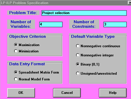
Here we shall just use the package to solve our simple project selection problem. If you wish to learn more about formulating and solving integer programs see here.
The package input for the problem presented above is given below.


with the solution being shown below.

Here we can see that the optimal decision is to choose to do projects 3 and 4.
Note that one advantage of formulating the problem in this structured manner (as a decision model, using variables, constraints and objective) is that we can investigate sensitivity very easily. For example you can see that in the above numeric solution we have chosen to do projects 3 and 4. This in fact means that we have spare capital available in years 1 and 2, but that all of our capital in year 3 is utilised. Suppose therefore (since all projects give a positive return) we wish to argue to higher management for this capacity constraint of 0.4 to be raised - how might you use the model you have developed to make your case for this capacity constraint to be raised?