OR-Notes are a series of introductory notes on topics that fall under the broad heading of the field of operations research (OR). They were originally used by me in an introductory OR course I give at Imperial College. They are now available for use by any students and teachers interested in OR subject to the following conditions.
A full list of the topics available in OR-Notes can be found here.
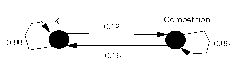
Consider the following problem: company K, the manufacturer of a breakfast cereal, currently has some 25% of the market. Data from the previous year indicates that 88% of K's customers remained loyal that year, but 12% switched to the competition. In addition, 85% of the competition's customers remained loyal to the competition but 15% of the competition's customers switched to K. Assuming these trends continue determine K's share of the market:
This problem is an example of a brand switching problem that often arises in the sale of consumer goods.
In order to solve this problem we make use of Markov chains or Markov processes (which are a special type of stochastic process). The procedure is given below.
Observe that, each year, a customer can either be buying K's cereal or the competition's. Hence we can construct a diagram as shown below where the two circles represent the two states a customer can be in and the arcs represent the probability that a customer makes a transition each year between states. Note the circular arcs indicating a "transition" from one state to the same state. This diagram is known as the state-transition diagram (and note that all the arcs in that diagram are directed arcs).
Given that diagram we can construct the transition matrix (usually denoted by the symbol P) which tells us the probability of making a transition from one state to another state. Letting:
we have the transition matrix P for this problem given by
      To state   1    2
From state   1 |0.88 0.12 |
             2 |0.15 0.85 |
Note here that the sum of the elements in each row of the transition matrix is one. Note also that the transition matrix is such that the rows are "From" and the columns are "To" in terms of the state transitions.
Now we know that currently K has some 25% of the market. Hence we have the row matrix representing the initial state of the system given by:
     State
     1     2
   [0.25, 0.75]
We usually denote this row matrix by s1 indicating the state of the system in the first period (years in this particular example). Now Markov theory tells us that, in period (year) t, the state of the system is given by the row matrix st where:
st = st-1(P) =st-2(P)(P) = ... = s1(P)t-1
We have to be careful here as we are doing matrix multiplication and the order of calculation is important (i.e. st-1(P) is not equal to (P)st-1 in general). To find st we could attempt to raise P to the power t-1 directly but, in practice, it is far easier to calculate the state of the system in each successive year 1,2,3,...,t.
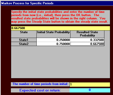
We already know the state of the system in year 1 (s1) so the state of the system in year two (s2) is given by:
s2 = s1P
= [0.25,0.75] |0.88 0.12 |
              |0.15 0.85 |
= [(0.25)(0.88) + (0.75)(0.15), (0.25)(0.12) + (0.75)(0.85)]
= [0.3325, 0.6675]
Note that this result makes intuitive sense, e.g. of the 25% currently buying K's cereal 88% continue to do so, whilst of the 75% buying the competitor's cereal 15% change to buy K's cereal - giving a (fractional) total of (0.25)(0.88) + (0.75)(0.15) = 0.3325 buying K's cereal.
Hence in year two 33.25% of the people are in state 1 - that is buying K's cereal. Note here that, as a numerical check, the elements of st should always sum to one.
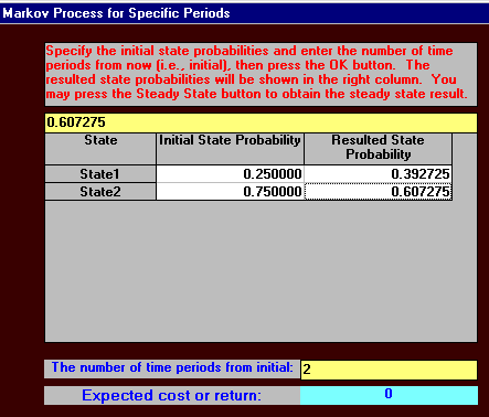
In year three the state of the system is given by:
s3 = s2P
= [0.3325, 0.6675] |0.88 0.12 |
                   |0.15 0.85 |
= [0.392725, 0.607275]
Hence in year three 39.2725% of the people are buying K's cereal.
Now it is plainly nonsense to suggest that we can predict to four decimal places K's market share in two years time - but the calculation has enabled us to get some insight into the change in K's share of the market over time that we otherwise might not have had.
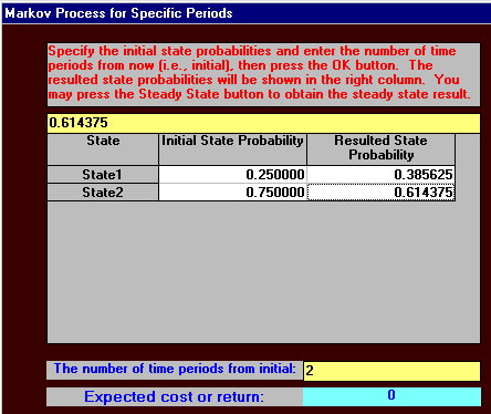
The above problem was solved using the package, the input being shown below.
The output is shown below, first after a single time period (year in this case), then for after two time periods.
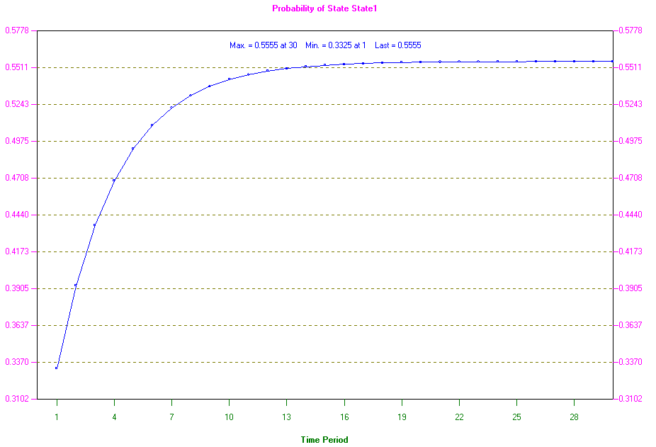
Using the package we can also graph the change in K's market share over time. This can be seen below. Note how (for this particular example) the market share rises steeply in the first few periods but then tails off and appears to reach a limit.
One advantage of using the package is that we can easily investigate changes. For example suppose, through a marketing/advertising campaign, that company K could increase the loyalty of their customers, specifically increase the transition probability from K to K by 0.01, i.e. to 0.89.
Now if K were to do this suppose we believe that the competition will respond with their own campaign and this will enable them to maintain loyalty amongst their own customers, with the Competition to Competition transition probability increasing from 0.85 to 0.86.
Will K have a larger or smaller (or the same) market share after two years in this case and what will be its market share?
Using the package we have:
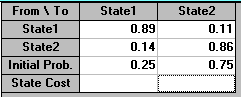
and
indicating that this situation will not improve K's market share in two years - as can be seen above this is now 38.5625% whereas before it was higher - 39.2725%. Knowing this without the effort and expense of a marketing campaign is obviously extremely valuable.
Recall that the question asked for K's share of the market in the long-run. This implies that we need to calculate st as t becomes very large (approaches infinity).
The idea of the long-run is based on the assumption that, eventually, the system reaches "equilibrium" (often referred to as the "steady-state") in the sense that st = st-1. This is not to say that transitions between states do not take place, they do, but they "balance out" so that the number in each state remains the same.
There are two basic approaches to calculating the steady-state:
[x1,x2] = [x1,x2] |0.88 0.12 |
                 |0.15 0.85 |
(and note also that x1 + x2 = 1). Hence we have three equations which we can solve.
Note here that we have used the word assumption above. This is because not all systems reach an equilibrium, e.g. the system with transition matrix
|0 1 |
|1 0 |
will never reach a steady-state.
Adopting the algebraic approach above for the K's cereal example we have the three equations:
x1 = 0.88x1 + 0.15x2
x2 = 0.12x1 + 0.85x2
x1 + x2 = 1
and rearranging the first two equations we get
0.12x1 - 0.15x2 = 0
0.12x1 - 0.15x2 = 0
x1 + x2 = 1
Note here that the equation x1 + x2 = 1 is essential. Without it we could not obtain a unique solution for x1 and x2. Solving we get x1 = 0.5556 and x2 = 0.4444
Hence, in the long-run, K's market share will be 55.56%.
A useful numerical check (particularly for larger problems) is to substitute the final calculated values back into the original equations to check that they are consistent with those equations.
The above problem was solved using the package, the output being shown below.
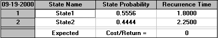
In the output shown above note:
The above analysis is plainly simplistic. We cannot pretend to have accurately predicted market shares into the future. Changing circumstances will change the transition matrix over time. However what the above analysis has given us is some insight that we did not have before. For example:
Such insights, based as they are on a quantitative analysis, can help us in decision making. For example, if we wanted K to have a market share of 35% in two years time we need do nothing (on current trends). If we wanted K to have a market share of 50% in two years time then, on current trends, we do need to do something. How much we need to change any given transition probability to achieve our target market share of 50% in two years time is easily calculated.
Moreover reflect on what all the TV/other media advertisements for consumer items are meant to do. For many items (since the total market demand is effectively stable, what is often called by economists a saturated market, "all the people who are going to buy are already buying") what such advertisements are meant to achieve is to alter consumer switching (transition) probabilities.You should be clear that transition probabilities need not be regarded as fixed numbers - rather they are often things that we can influence/change.
Nowadays many supermarkets in the UK have their own "loyalty cards" which are swiped through the checkout at the same time as a customer makes their purchases. These provide a mass of detailed information from which supermarkets (or others) can deduce brand switching transition matrices:
Now consider how many different products/types of products a supermarket sells. The data they are gathering on their databases through the use of loyalty cards can be extremely valuable to them.
Note too that the availability of such data enables more detailed models to be constructed. For example in the cereal problem we dealt with above the competition was represented by just one state. With more detailed data that state could be disaggregated into a number of different states - maybe one for each competitor brand of cereal. If we have n states then we need n2 transition probabilities. Estimating these probabilities is easy if we have access to a supermarket database which tells us from individual consumer data whether people switched or not, and if so to what.
Also we could have different models for different segments of the market - maybe brand switching is different in rural areas from brand switching in urban areas for example. Families with young children would obviously constitute another important brand switching segment of the cereal market.
Note here that if we wish to investigate brand switching in a numeric way then transition probabilities are key. Unless we can get such numbers nothing numeric is possible.
Consider now how, in the absence of readily available information on brand switching as gathered by a supermarket (e.g. because we cannot afford the price the supermarkets are asking for such information), we might get information as to transition probabilities. One way, indeed this is how this was done before loyalty cards, is to survey customers individually. Someone physically stands outside the supermarket and asks shoppers about their current purchases and their previous purchases. Whilst this can be done it is plainly expensive - particularly if we need to achieve a reasonable geographic coverage that is regularly updated as time passes.
Both of the above ways of estimating transition matrices - buying electronic information and manual surveys - cost money. There is however one way that is effectively COST FREE although, as will become apparent below, it does involve some intellectual effort. This involves estimating the transition probabilities (i.e. the entire transition matrix) from the observed market shares. We illustrate how this can be done below.
Consider a simple two state example involving two companies. Suppose that the market shares in the first period are [0.3,0.7] and in the next period they are [0.2,0.8] - what then would you estimate the transition matrix to be?
Letting the transition matrix be:
| p1  1-p1|
|1-p2  p2 |
we have that
[0.2,0.8] = [0.3,0.7]| p1  1-p1|
                     |1-p2  p2 |
so that we have
0.2 = 0.3p1 + 0.7(1-p2)
0.8 = 0.3(1-p1) + 0.7p2
which give
-0.5 =  0.3p1 - 0.7p2
 0.5 = -0.3p1 + 0.7p2
and as these two equations are identical (one is the other with the sign changed) we have no unique way of determining values for p1 and p2.
To overcome this one approach that will yield valid numeric values for p1 and p2 is to say that whatever the transition matrix is, we would like the diagonal entries (p1 and p2) to be as large as possible. This is equivalent to saying that we believe that the combined probabilities of making a transition away from the original states should be as small as possible. This is equivalent to saying that consumers/customers are loyal and tend to stay with what they know ("brand inertia"). Hence we can formulate the problem of determining p1 and p2 as
maximise p1 + p2
subject to
0.5 = -0.3p1 + 0.7p2
0 <= p1 <= 1
0 <= p2 <= 1
where we have added restrictions on p1 and p2, namely that they must lie between zero and one. Now this problem is just a linear programming (LP) problem that can be easily solved using the package, as below.
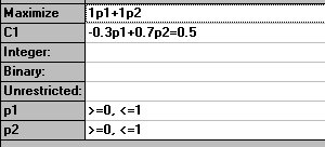
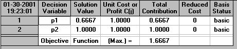
so that the solution is p1=(2/3) and p2=1. It is easily checked that these values satisfy the equation 0.5 = -0.3p1 + 0.7p2. Hence our transition matrix is:
| 2/3 1/3 |
| 0    1  |
Note here that, as our original equation 0.5 = -0.3p1 + 0.7p2 implied, there are many possible transition matrices that exactly correspond to the observed market shares. What we have done here in producing the transition matrix shown above is to choose one of these transition matrices as derived from the solution to an optimisation problem.
To extend our example suppose that the observed market shares are
first  [0.3,0.7]
then   [0.2,0.8]
then   [0.15,0.85]
then   [0.13,0.87]
where the first two periods here are as in the example dealt with above. What would you estimate the transition matrix to be now?
Obviously we could take each successive pair of market shares and use exactly the same approach as above, deriving transition matrices that apply between each and every time period.
We have done this above for the first two periods and obtained
| 2/3 1/3 |
| 0    1  |
If we do this for periods 2 and 3 we have
[0.15,0.85] = [0.2,0.8]| p1  1-p1|
                       |1-p2  p2 |
for which the corresponding linear equation is
0.15 = 0.2p1 + 0.8(1-p2)
i.e. -0.65 = 0.2p1 - 0.8p2
which following the same approach as before leads to the linear program
maximise p1 + p2
subject to
-0.65 = 0.2p1 - 0.8p2
0 <= p1 <= 1
0 <= p2 <= 1
for which the solution is p1=(3/4) and p2=1. It is easily checked that these values satisfy the equation -0.65 = 0.2p1 - 0.8p2. Hence our transition matrix is:
| 3/4 1/4 |
| 0    1  |
So we now have a different transition matrix to the one we derived when we considered just the first two periods! So this approach, whilst possible, leads to conceptual difficulties - did the transition matrix really change between periods or do we need a better way of estimating it?
Suppose we want a SINGLE transition matrix that, when applied over all time periods, best captures the observed market shares - how can we find it?
Well, as before, let us assume that this single transition matrix is
| p1  1-p1|
|1-p2  p2 |
and recall that we have
first  [0.3,0.7]
then   [0.2,0.8]
then   [0.15,0.85]
then   [0.13,0.87]
then, from the initial market shares of [0.3,0.7] we have that the market shares in the next period are
[0.3,0.7]| p1  1-p1|
         |1-p2  p2 |
= [0.3p1 + 0.7(1-p2), 0.3(1-p1) + 0.7p2] - as against the observed market shares in this period of [0.2,0.8]
For the next period, starting from [0.2,0.8] we have
[0.2,0.8]| p1  1-p1|
         |1-p2  p2 |
= [0.2p1 + 0.8(1-p2), 0.2(1-p1) + 0.8p2] - as against the observed market shares in this period of [0.15,0.85]
For the next period, starting from [0.15,0.85] we have
[0.15,0.85]| p1  1-p1|
           |1-p2  p2 |
= [0.15p1 + 0.85(1-p2), 0.15(1-p1) + 0.85p2] - as against the observed market shares in this period of [0.13,0.87]
Hence we can construct a table as below:
Time  State   Calculated          Observed
1     1       0.3p1 + 0.7(1-p2)    0.2
      2       0.3(1-p1) + 0.7p2    0.8
2     1       0.2p1 + 0.8(1-p2)    0.15
      2       0.2(1-p1) + 0.8p2    0.85
3     1       0.15p1 + 0.85(1-p2)  0.13
      2       0.15(1-p1) + 0.85p2  0.87
Plainly it would be ideal if we could choose values for p1 and p2 such that each of the calculated expressions EXACTLY matches the observed market shares i.e. choose p1 and p2 such that
0.3p1 + 0.7(1-p2)   = 0.2
0.3(1-p1) + 0.7p2   = 0.8
0.2p1 + 0.8(1-p2)   = 0.15
0.2(1-p1) + 0.8p2   = 0.85
0.15p1 + 0.85(1-p2) = 0.13
0.15(1-p1) + 0.85p2 = 0.87
The above are all linear equations so we can approach solving them via an LP as before - simply
maximise p1 + p2
subject to
0.3p1 + 0.7(1-p2)   = 0.2
0.3(1-p1) + 0.7p2   = 0.8
0.2p1 + 0.8(1-p2)   = 0.15
0.2(1-p1) + 0.8p2   = 0.85
0.15p1 + 0.85(1-p2) = 0.13
0.15(1-p1) + 0.85p2 = 0.87
0 <= p1 <= 1
0 <= p2 <= 1
If we solve this LP numerically we will find that the problem is infeasible - i.e. there are no values for p1 and p2 that satisfy the above equations. Hence we seem to have reached an impasse.
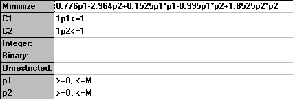
One way forward so as to choose values for p1 and p2 is again to solve an optimisation problem, but where this time we minimise the squared difference between the calculated state in each time period and the observed state, i.e. minimise the sum of squared errors (a common approach in parameter estimation). Hence we need to solve:
minimise
[0.3p1 + 0.7(1-p2)   - 0.2]2 +
[0.3(1-p1) + 0.7p2   - 0.8]2 +
[0.2p1 + 0.8(1-p2)   - 0.15]2 +
[0.2(1-p1) + 0.8p2   - 0.85]2 +
[0.15p1 + 0.85(1-p2) - 0.13]2 +
[0.15(1-p1) + 0.85p2 - 0.87]2
subject to:
0 <= p1 <= 1
0 <= p2 <= 1
Simplifying this objective we have
minimise [0.3p1 - 0.7p2 + 0.5]2 + [-0.3p1 + 0.7p2 - 0.5]2 + [0.2p1 - 0.8p2 + 0.65]2 + [-0.2p1 + 0.8p2 - 0.65]2 + [0.15p1 - 0.85p2 + 0.72]2 + [-0.15p1 + 0.85p2 - 0.72]2
which is
minimise 2[0.3p1 - 0.7p2 + 0.5]2 + 2[0.2p1 - 0.8p2 + 0.65]2 + 2[0.15p1 - 0.85p2 + 0.72]2
Obviously we need to simplify this expression - in doing so note that any constant terms can be ignored, since they cannot affect the values for p1 and p2 chosen, merely the value of the objective function. In a similar fashion we can drop the common multiplier of 2 associated with each of the three terms in this objective.
After simplification we have the problem:
minimise 0.1525[p1]2 + 1.8525[p2]2 - 0.995p1p2 + 0.776p1 - 2.964p2 subject to 0<= p1<=1 and 0<= p2<= 1
This is a nonlinear (quadratic) program that can be easily solved using the package as below:
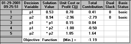
Hence we can see that the solution is p1=0.53, p2=0.94 and hence the transition matrix is
| 0.53 0.47 |
| 0.06 0.94 |
Using these values of p1=0.53 and p2=0.94 we have:
Time  State   Calculated          Estimated  Observed
1     1       0.3p1 + 0.7(1-p2)    0.201      0.2
      2       0.3(1-p1) + 0.7p2    0.799      0.8
2     1       0.2p1 + 0.8(1-p2)    0.142      0.15
      2       0.2(1-p1) + 0.8p2    0.846      0.85
3     1       0.15p1 + 0.85(1-p2)  0.131      0.13
      2       0.15(1-p1) + 0.85p2  0.870      0.87
which appears to be a very good estimation, via a single transition matrix, of the observed market shares.
Be clear here - what we have done above is to find, in a logical consistent systematic fashion, a transition matrix that "best fits" the observed market shares - that transition matrix may (or may not) correspond to the transition probabilities which we would find were we to survey customers or gather electronic information in the real-world. Hopefully though the transition matrix found will provide insight that we did not have before.
Here the transition matrix we have derived above does give us further insight into the situation - we can see for example that customers of company 2 (state 2) are very loyal (94% remain with that company at each time period). Customers of company 1 (state 1) are not loyal on the other hand - only 53% remaining with company 1 at each time period - almost equivalent to customers tossing a coin to decide whether to go with company 1 or company 2. This numeric insight with respect to customer loyalty may be one that we could not have gained simply by looking at the observed market shares of
first  [0.3,0.7]
then   [0.2,0.8]
then   [0.15,0.85]
then   [0.13,0.87]
and obviously suggests a way in which company 1 might try to gain market share (or arrest their declining market share) - namely increase customer loyalty.
To consolidate your knowledge of Markov processes consider the following example. Suppose the chip industry is controlled by four companies: Crispy, Crunchy, Mushy and Scrunchy. If customers buy either Crispy or Crunchy they never buy another brand. If they buy Mushy the probabilities that they will buy Crispy, Crunchy, Mushy and Scrunchy next month are 0.45, 0.4, 0.05 and 0.1 respectively. If they buy Scrunchy the probabilities that they will buy Crispy, Crunchy, Mushy and Scrunchy next month are 0.1, 0.2, 0.3 and 0.4 respectively.
The state-transition diagram for this problem is shown below.
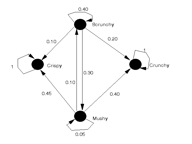
Letting
we have that
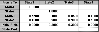
P = | 1    0   0    0   |
    | 0    1   0    0   |
    | 0.45 0.4 0.05 0.1 |
    | 0.1  0.2 0.3  0.4 |
and s1 = [0.2, 0.3, 0.3, 0.2]
Note here that the states corresponding to Crispy and Crunchy are absorbing states (states which, once reached, cannot be left). States which are non-absorbing are often called transient states.
Hence the state of the system in the second month s2 = s1P
= [0.2, 0.3, 0.3, 0.2]| 1    0   0    0   |
                      | 0    1   0    0   |
                      | 0.45 0.4 0.05 0.1 |
                      | 0.1  0.2 0.3  0.4 |
= [0.355, 0.46, 0.075, 0.11]
The state of the system in the third month s3 = s2P
= [0.355, 0.46, 0.075, 0.11]| 1    0   0    0   |
                            | 0    1   0    0   |
                            | 0.45 0.4 0.05 0.1 |
                            | 0.1  0.2 0.3  0.4 |
= [0.39975, 0.512, 0.03675, 0.0515]
The above problem was solved using the package, the input being shown below.
The output is shown below. For simplicity we have shown the state of the system after 20 time periods. It will be seen that (as we would expect) all the buyers end up in one of the two absorbing states.
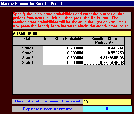
Note here that, if absorbing states are present, the mathematics needed to calculate the long-run system state is MUCH MORE complicated than the approach given before that worked when absorbing states were not present. Indeed, as a reflection of this, the package refuses to calculate a steady state for this example.
To see why this is so try to apply the same method as we used above when we had no absorbing states - letting the long-run system state be [x1,x2,x3,x4] we have
[x1,x2,x3,x4] = [x1,x2,x3,x4]| 1    0   0    0   |
                           | 0    1   0    0   |
                           | 0.45 0.4 0.05 0.1 |
                           | 0.1  0.2 0.3  0.4 |
where x1 + x2 + x3 + x4 = 1
Taking the last two equations from this matrix equation we get
x3 = 0.05x3 + 0.3x4
x4 = 0.1x3 + 0.4x4
i.e. x3 = (0.3/0.95)x4 and x3 = (0.6/0.1)x4 and the only values of x3 and x4 that satisfy these two equations are x3=x4=0 (as we might have suspected). Using x3=x4=0 the remaining equations from above become
x1 = x1
x2 = x2
x1 + x2 = 1
which are somewhat difficult to solve !
Any problem for which a state-transition diagram can be drawn can be analysed using the approach given above.
The advantages and disadvantages of using Markov theory include:
One interesting application of Markov processes that I know of concerns the Norwegian offshore oil/gas industry. In Norway a state body, the Norwegian Petroleum Directorate, (together with the Norwegian state oil company (STATOIL)), have a large role to play in planning the development of oil/gas offshore facilities.
The essential problem the Norwegian Petroleum Directorate has is how to plan pipelines/field startup/production so as to maximise the contribution to the Norwegian economy over time. Here the time scales are very long, typically 30 to 50 years.
There is decision flexibility with respect to a number of items, e.g.
The objective is to maximise the benefit to the Norwegian economy over time.
Of critical importance is the oil price - yet we cannot sensibly forecast this with accuracy for the length of time, 30 to 50 years, we need to consider.
To overcome this problem they model oil price as a Markov process with three price levels (states), corresponding to optimistic, most likely and pessimistic scenarios. They also specify the probabilities of making a transition between states each time period (year). Different transition matrices can be used for different time scales (e.g. different matrices for the near, medium and far future).
Whilst this is plainly a simple approach it does have the advantage of capturing the uncertainty about the future in a model that is relatively easy to understand and apply.
Population modelling studies (where we have objects which "age") are also an interesting application of Markov processes:
Some more markov processes examples can be found here.