OR-Notes are a series of introductory notes on topics that fall under the broad heading of the field of operations research (OR). They were originally used by me in an introductory OR course I give at Imperial College. They are now available for use by any students and teachers interested in OR subject to the following conditions.
A full list of the topics available in OR-Notes can be found here.
When formulating LP's we often found that, strictly, certain variables should have been regarded as taking integer values but, for the sake of convenience, we let them take fractional values reasoning that the variables were likely to be so large that any fractional part could be neglected. Whilst this is acceptable in some situations, in many cases it is not, and in such cases we must find a numeric solution in which the variables take integer values.
Problems in which this is the case are called integer programs (IP's) and the subject of solving such programs is called integer programming (also referred to by the initials IP).
IP's occur frequently because many decisions are essentially discrete (such as yes/no, go/no-go) in that one (or more) options must be chosen from a finite set of alternatives.
Note here that problems in which some variables can take only integer values and some variables can take fractional values are called mixed-integer programs (MIP's).
As for formulating LP's the key to formulating IP's is practice. Although there are a number of standard "tricks" available to cope with situations that often arise in formulating IP's it is probably true to say that formulating IP's is a much harder task than formulating LP's.
We consider an example integer program below.
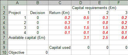
There are four possible projects, which each run for 3 years and have the following characteristics.
                         Capital requirements (£m)
Project   Return (£m)    Year   1     2     3
1         0.2                   0.5   0.3   0.2
2         0.3                   1.0   0.8   0.2
3         0.5                   1.5   1.5   0.3
4         0.1                   0.1   0.4   0.1
Available capital (£m)          3.1   2.5   0.4
We have a decision problem here: Which projects would you choose in order to maximise the total return?
We follow the same approach as we used for formulating LP's - namely:
We do this below and note here that the only significant change in formulating IP's as opposed to formulating LP's is in the definition of the variables.
Here we are trying to decide whether to undertake a project or not (a "go/no-go" decision). One "trick" in formulating IP's is to introduce variables which take the integer values 0 or 1 and represent binary decisions (e.g. do a project or not do a project) with typically:
Such variables are often called zero-one or binary variables
To define the variables we use the verbal description of
xj = 1 if we decide to do project j (j=1,...,4)
   = 0 otherwise, i.e. not do project j (j=1,...,4)
Note here that, by definition, the xj are integer variables which must take one of two possible values (zero or one).
The constraints relating to the availability of capital funds each year are
0.5x1 + 1.0x2 + 1.5x3 + 0.1x4
<= 3.1 (year 1)
0.3x1 + 0.8x2 + 1.5x3 + 0.4x4
<= 2.5 (year 2)
0.2x1 + 0.2x2 + 0.3x3 + 0.1x4
<= 0.4 (year 3)
To maximise the total return - hence we have
maximise 0.2x1 + 0.3x2 + 0.5x3 + 0.1x4
This gives us the complete IP which we write as
maximise 0.2x1 + 0.3x2 + 0.5x3 + 0.1x4
subject to
0.5x1 + 1.0x2 + 1.5x3 + 0.1x4
<= 3.1
0.3x1 + 0.8x2 + 1.5x3 + 0.4x4
<= 2.5
0.2x1 + 0.2x2 + 0.3x3 + 0.1x4
<= 0.4
xj = 0 or 1 j=1,...,4
Note:
Extensions to this basic problem include:
How to amend our basic IP to deal with such extensions is given here.
In fact note here that integer programming/quantitative modelling techniques are increasingly being used for financial problems.
Solution methods for IP's can be categorised as:
An optimal algorithm is one which (mathematically) guarantees to find the optimal solution.
It may be that we are not interested in the optimal solution:
In such cases we can use a heuristic algorithm - that is an algorithm that should hopefully find a feasible solution which, in objective function terms, is close to the optimal solution. In fact it is often the case that a well-designed heuristic algorithm can give good quality (near-optimal) results.
For example a heuristic for our capital budgeting problem would be:
Applying this heuristic we would choose to do just project 1 and project 2, giving a total return of 0.5, which may (or may not) be the optimal solution.
Note here that the methods presented below are suitable for solving both IP's (all variables integer) and MIP's (mixed-integer programs - some variables integer, some variables allowed to take fractional values).
We shall deal with just two general purpose (able to deal with any IP) optimal solution algorithms for IP's:
We consider each of these in turn below.
Unlike LP (where variables took continuous values (>=0)) in IP's (where all variables are integers) each variable can only take a finite number of discrete (integer) values.
Hence the obvious solution approach is simply to enumerate all these possibilities - calculating the value of the objective function at each one and choosing the (feasible) one with the optimal value.
For example for the capital budgeting problem considered above there are 24=16 possible solutions. These are:
x1 x2  x3 x4
0  0  0  0  do no projects

0  0  0  1  do one project
0  0  1  0
0  1  0  0
1  0  0  0

0  0  1  1  do two projects
0  1  0  1
1  0  0  1
0  1  1  0
1  0  1  0
1  1  0  0

1  1  1  0  do three projects
1  1  0  1
1  0  1  1
0  1  1  1

1  1  1  1  do four projects
Hence for our example we merely have to examine 16 possibilities before we know precisely what the best possible solution is. This example illustrates a general truth about integer programming:
What makes solving the problem easy when it is small is precisely what makes it become very hard very quickly as the problem size increases
This is simply illustrated: suppose we have 100 integer variables each with 2 possible integer values then there are 2x2x2x ... x2 = 2100 (approximately 1030) possibilities which we have to enumerate (obviously many of these possibilities will be infeasible, but until we generate one we cannot check it against the constraints to see if it is feasible or not).
This number is plainly too many for this approach to solving IP's to be computationally practicable. To see this consider the fact that the universe is around 1010 years old so we would need to have considered 1020 possibilities per year, approximately 4x10¹² possibilities per second, to have solved such a problem by now if we started at the beginning of the universe.
Be clear here - conceptually there is not a problem - simply enumerate all possibilities and choose the best one. But computationally (numerically) this is just impossible.
IP nowadays is often called "combinatorial optimisation" indicating that we are dealing with optimisation problems with an extremely large (combinatorial) increase in the number of possible solutions as the problem size increases.
Capital budgeting solution - using Solver
Below we solve the capital budgeting problem with the Solver add-in that comes with Microsoft Excel.
If you click here you will be able to download an Excel spreadsheet called ip.xls that already has the IP we are considering set up.
Take this spreadsheet and look at Sheet A. You should see the problem we considered above set out as:
Here we have set up the problem with the decisions (the zero-one variables) being shown in cells B3 to B6. The capital used in each of the three years is shown in cells D9 to F9 and the objective (total return) is shown in cell B10 (for those of you interested in Excel we have used SUMPRODUCT in cells D9 to F9 and B10 as a convenient way of computing the sum of the product of two sets of cells).
Doing Tools and then Solver you will see:
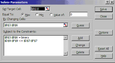
where B10 is to be maximised (ignore the use of $ signs here - that is a technical Excel issue if you want to go into it in greater detail) by changing the decision cells B3 to B6 subject to the constraints that these cells have to be binary (zero-one) and that D9 to F9 are less than or equal to D7 to F7, the capital availability constraints.
Clicking on Options on the above Solver Parameters box you will see:

showing that we have ticked Assume Linear Model and Assume Non-Negative.
Solving we get:
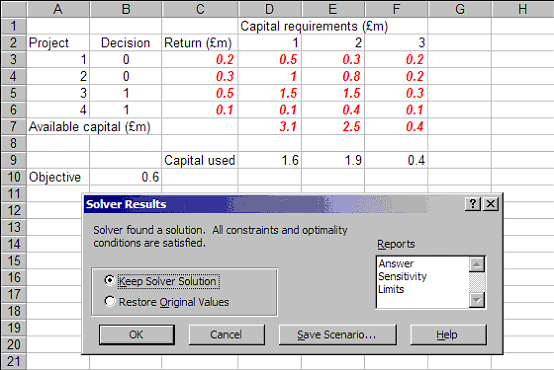
indicating that the optimal decision (the decision that achieves the maximum return of 0.6 shown in cell B10) is to do projects 3 and 4 (the decision variables are one in cells B5 and B6, but not to do projects 1 and 2 (the decision variables are zero in cells B3 and B4).