OR-Notes are a series of introductory notes on topics that fall under the broad heading of the field of operations research (OR). They were originally used by me in an introductory OR course I give at Imperial College. They are now available for use by any students and teachers interested in OR subject to the following conditions.
A full list of the topics available in OR-Notes can be found here.
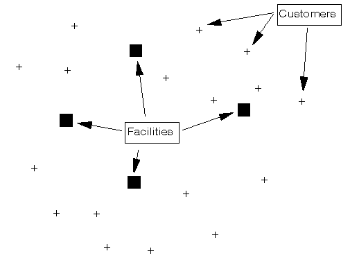
The general facility location problem is: given a set of facility locations and a set of customers who are served from the facilities then:
Typically here facilities are regarded as "open" (used to serve at least one customer) or "closed" and there is a fixed cost which is incurred if a facility is open. Which facilities to have open and which closed is our decision.
Below we show a graphical representation of the problem.
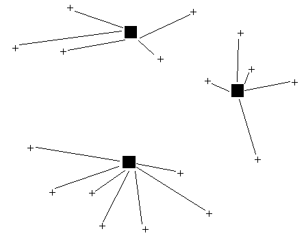
One possible solution is shown below.
Other factors often encountered here:
The problems of facility size and facility location are very closely linked and should be considered simultaneously. In fact the package used here disregards (for reasons of simplicity) the problem of facility size and deals only with facility location.
We shall illustrate the problem of facility location by means of an example.
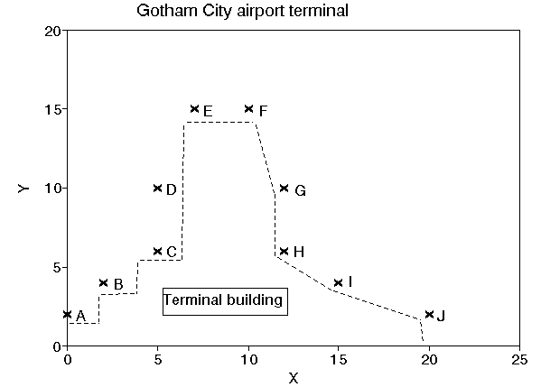
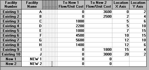
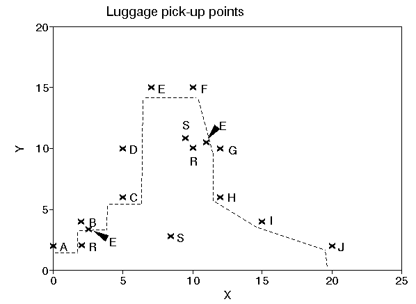
At Gotham City airport terminal there are 10 arrival gates (A to J respectively). A pictorial representation of the terminal is given below with the location of the gates being:
Gate x coordinate y coordinate
A       0              2
B       2              4
C       5              6
D       5              10
E       7              15
F       10             15
G       12             10
H       12             6
I       15             4
J       20             2
Luggage from arriving flights is unloaded at these gates and moved to a passenger luggage pick-up point.
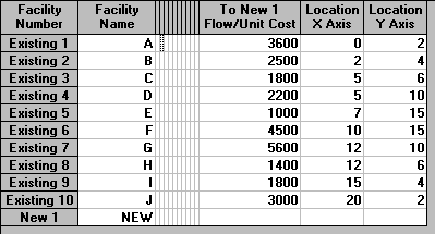
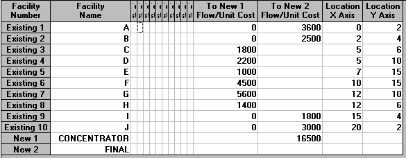
It is estimated that the number of pieces of luggage arriving per day at each gate (A to J respectively) is: 3600, 2500, 1800, 2200, 1000, 4500, 5600, 1400, 1800 and 3000 respectively.
Where should the passenger luggage pick-up point be located in order to minimize movement of luggage?
In order to logically locate the passenger luggage pick-up point we need to make use of the amount of luggage flowing from the gates to the pick-up point. Logically a gate from which there is a large flow should be nearer to the pick-up point than a gate with a small flow.
Informally therefore we would like to position the pick-up point so as to minimise the sum over all gates g (distance between g and the pick-up point) multiplied by (flow between g and the pick-up point).
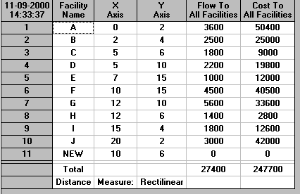
This approach to choosing the location of the pick-up point is precisely the approach used by the facility location module in the package. Typically in such location problems we are concerned with a load-distance score (the product of load and distance for all points). The initial input to the package for this problem is shown below.

Note here the package terminology is somewhat peculiar:
In order to enter the data relating to the gates we can ignore the columns in the package input that are concerned with flows between existing facilities - here all flows are from the existing facilities to the new facility.
Note here that in solving the problem we need to specify the appropriate distance model.
This is because as we do not yet know where the new facility (luggage pick-up point) is to be we cannot specify the distance between it and the gates without a general expression for calculating the distance between two locations. If (xi,yi) and (xj,yj) represent the coordinates of two locations i and j then the distance model measures can be:
The rectilinear distance measure is often used for factories, American cities, etc which are laid out in the form of a rectangular grid. For this reason it is sometimes called the Manhattan distance measure. The Euclidean distance measure is used where genuine straight line travel is possible. The squared Euclidean distance measure is used where straight line travel is possible but where we wish to discourage excessive distances (squaring a large distance number results in an even larger distance number and recall that we use the distance number in the objective which we are trying to minimise).
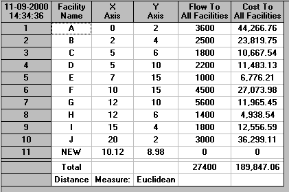
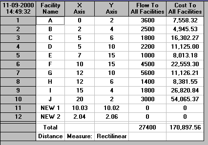
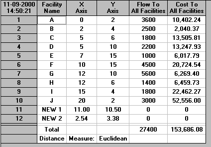
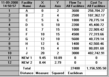
The output from the package for each of the distance measures is shown below.
Rectilinear
Euclidean
Squared Euclidean
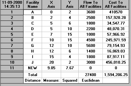
From the package output we can see that the location for the luggage pick-up point should be:
Distance measure       x coordinate   y coordinate
Rectilinear            10             6
Euclidean              10.12          8.98
Squared Euclidean      9.05           7.67
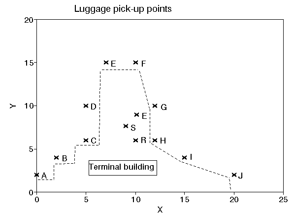
The picture below shows these three possible locations with respect to the terminal (labelled R, E and S for rectilinear, Euclidean and squared Euclidean respectively).
Note here that (in reality) the initial choice of distance measure is often between rectilinear and Euclidean (based upon the technology of how the luggage flows within the terminal). If the luggage flows in an Euclidean (straight-line) manner then choosing to use squared Euclidean, rather than Euclidean, penalises excessively long distances.
One point to note about the above picture is that we are not really interested in determining positions down to the nearest millimetre (the data is probably not accurate enough anyway!). Instead we are using the package to get an indication of the approximate region where it would be sensible to site a luggage pick-up point.
Note too that the package uses a "centre of gravity" approach to decide where to locate a single pick-up point.
Suppose now we are interested in having two luggage pick-up points. We have two types of decisions:
Ideally we would like a way of automatically solving both these decision problems simultaneously (since obviously location affects allocation and vice-versa).
The package we are using cannot do this. Instead we must ourselves decide the allocation and allow the package to solve to produce appropriate locations.
However more sophisticated packages can solve both decisions simultaneously.
Suppose therefore that we make an (arbitrary) allocation decision, based upon the map of the terminal, namely that we will have one luggage pick-up point dealing with gates C to H (inclusive) and the other dealing with gates A, B, I and J.
With this allocation decision made we can solve the problem using the package, the input being shown below. Note here that in this input we have made new facility number 1 the luggage pick-up point for gates C to H (inclusive) and new facility number 2 the luggage pick-up point for gates A, B, I and J.
Note the cells associated with flows between New Facilities. This is for flows between new facilities, whose locations we do not yet know. For example, we could be moving luggage using a concentrator system. Luggage flows to a central point (new facility, a concentrator point) before being passed onward to a collection point (new facility). In such a case the flow from the concentrator point to the collection point would need to be given in this matrix.
The output from the package for each of the three distance measures is shown below.
Rectilinear
Euclidean
Squared Euclidean
From this output we can see that the locations for the luggage pick-up points should be:
Distance measure       Facility     x coordinate   y coordinate
Rectilinear            1            10.03          10.02
                       2            2.04           2.06
Euclidean              1            11.00          10.50
                       2            2.54           3.38
Squared Euclidean      1            9.45           10.89
                       2            8.44           2.79
The picture below shows all these locations with respect to the terminal
(labelled R, E and S for rectilinear, Euclidean and squared Euclidean respectively).
Suppose now that in the example we just considered the luggage pick-up point for gates C to H (inclusive) is merely acting as a concentrator, concentrating luggage before passing it to the other pick-up point, which collects luggage from gates A,B, I and J directly. In this system all passengers see is a single pick-up point at which they collect their luggage. To locate this concentrator (and the final pick-up point) we make use of flows between new facilities. Here the total amount of luggage collected from C to H will flow to the final pick-up point from this intermediate concentrator. This will total 1800+2200+1000+4500+5600+140 =16500 pieces of luggage. Hence the input to the package is:
The solutions are:
Rectilinear
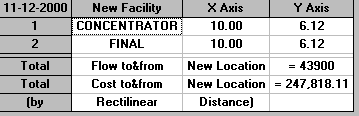
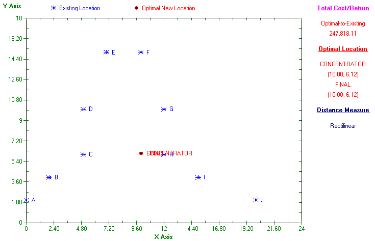
So in this case the final and concentrator locations coincide.
Euclidean


So in this case the final and concentrator locations are near to each other.
Squared Euclidean
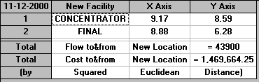
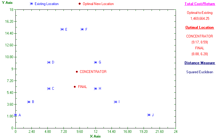
So in this case the final and concentrator locations are not particularly close to each other.
Technically the approach used above for location, where any point is a potential location for a new facility, is called the infinite set approach.
More commonly nowadays location studies are done using a feasible set approach. With this approach there are a finite set of alternatives for the new facilities and the problem is to choose from these alternatives the best subset to service a known set of customers (existing facilities in the terminology of the package used above). The advantage of this approach is that it can take explicit account of items such as fixed costs and capacities associated with facilities (i.e. items connected with facility size), as well as the issue of deciding the allocation of customers to facilities.
Location models based upon the feasible set approach typically use integer programming. More about such models can be found here.
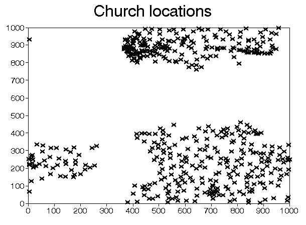
One example of a facility location problem that I have worked on was to do with church location for Church of England churches. The idea here was to investigate which churches could best be closed.
For the purposes of this study a 100 kilometre square to the north-east of London was chosen. An obvious first question is How many churches are there in this area and where are they? Alas the organisation did not seem too sure of the answers to this question. Eventually we consulted maps of the area and came to the conclusion that we thought there were 504 (Church of England) churches in this area. A plot of the location of these churches is shown below (church positions to one-tenth of a kilometre). You can see that they are clustered together in a number of distinct areas.
Now if a church (facility) is to be closed then logically we should consider information like
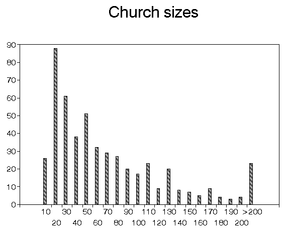
Unfortunately this was an extremely data-poor environment. The only data (aside from the above location data) we had was the average congregation (attendance) size for each of the 504 churches. This data is plotted below as a histogram. You can see that the average congregation size for a significant number of churches is very small.
We concluded that we had to work with the limited data we had, rather than attempt to discover data for 504 different churches, effectively an impossible task.
The approach we decided upon was to say that if a church was closed its congregation was displaced to their nearest open church. This leads naturally to the idea of displacement distance - defined to be congregation size multiplied by distance they are displaced. Our problem therefore is to choose the churches to close so as to minimise total displacement distance.
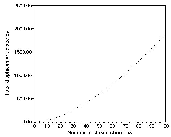
To solve this problem we took a simple interchange heuristic from the literature and coded it. The effect of closing churches in terms displacement distance (measured in people kilometres) is shown below. You can see that as more churches are closed the total displacement distance increases.
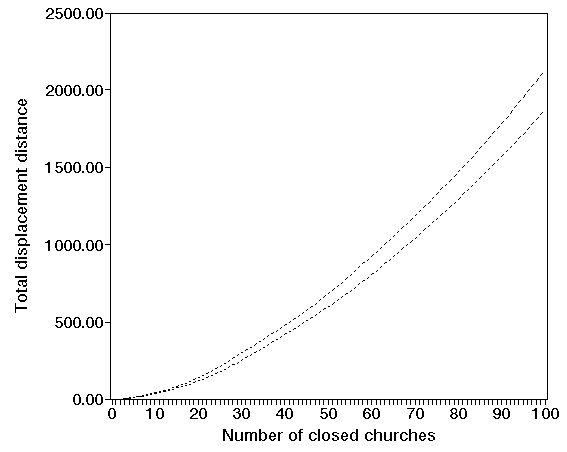
One complication to this study was that closer examination of the data revealed a number of churches very close to each other (say within 0.5 of a kilometre of each other) but with relatively large congregations. The algorithm attempted to close one of these churches (displacing the congregation to the other). Now all churches, even within the Church of England, are not the same in terms of the type of church service which they offer. Some are more evangelical, some more traditional, etc. It seemed likely that two churches very close to each other, but both with large congregations, were offering a different type of church service, so closing one and displacing the congregation to the other would not be satisfactory in practice.
We therefore modified our algorithm to ensure that no churches with a congregation of 50 or more could be closed (i.e. only "small" churches with a congregation less than 50 could be closed). The effect of this upon total displacement distance can be seen in the diagram below. In that diagram the lower line is as above (all churches available for closure) and the upper line is when only small churches can be closed.
A free package to help solve a variety of location problems is available here.