OR-Notes are a series of introductory notes on topics that fall under the broad heading of the field of operations research (OR). They were originally used by me in an introductory OR course I give at Imperial College. They are now available for use by any students and teachers interested in OR subject to the following conditions.
A full list of the topics available in OR-Notes can be found here.
Materials requirements planning, referred to by the initials MRP, is a technique which assists a company in the detailed planning of its production. Recall here that the master production schedule sets out an aggregate plan for production. MRP translates that aggregate plan into an extremely detailed plan
We shall introduce MRP by means of an example.
The production manager at Aldershot Manufacturing wishes to develop a materials requirements plan for producing chairs over an 8 week period. She estimates that the lead time between releasing an order to the shop floor and producing a finished chair is 2 weeks. The company currently has 260 chairs in stock and no safety stock (safety stock is stock held in reserve to meet customer demand if necessary). The forecast customer demand is for 150 chairs in week 1, 70 in week 3, 175 in week 5, 90 in week 7 and 60 in week 8.
It helps to understand what is going on if we write out, over time, the demand for chairs as below.
                     Week  1    2    3    4    5    6    7    8
Demand                   150    0   70    0  175    0   90   60
On-hand at end of week   110
Order                      ?    ?    ?    ?    ?    ?    ?    ?
Here we have shown the demand in each of the eight weeks, initially we have 260 chairs available so if these are used to meet the demand of 150 in week 1 we have 260-150 = 110 left on-hand (i.e. in stock) at the end of the week. Plainly we will need to order some more chairs in order to meet all of the forecast future demand over the 8 week planning period.
Conceptually therefore we face two related decisions about ordering:
You can think of asking yourself the question, in each and every period, should I order in this period and if so how much?
For the moment suppose we order nothing in week 1, nothing in week 2, etc. The situation by the time we reach the end of week 5 will be as below:
                     Week  1    2    3    4    5    6    7    8
Demand                   150    0   70    0  175    0   90   60
On-hand at end of week   110  110   40   40 -135
Order                      ?    ?    ?    ?    ?    ?    ?    ?
If we are to avoid a stockout in week 5 we plainly need to order at least 135 chairs. Now we know that the lead time between ordering a chair and receiving it is 2 weeks. Therefore to avoid a stockout in week 5 we must have ordered 135 chairs either in week 3, or in any week before week 3. In other words ordering
would each ensure that we have sufficient chairs available to meet forecast demand in week 5.
If we order these chairs earlier than week 3 we will be carrying extra inventory (stock) for a number of periods and, as we know, carrying stock costs money. It would seem appropriate therefore to order 135 chairs in week 3. This will give:
                     Week  1    2    3    4    5    6    7    8
Demand                   150    0   70    0  175    0   90   60
On-hand at end of week   110  110   40   40    0
Order                      0    0  135    ?    ?    ?    ?    ?
Continuing on in the same manner we get:
                     Week  1    2    3    4    5    6    7    8
Demand                   150    0   70    0  175    0   90   60
On-hand at end of week   110  110   40   40    0    0  -90
Order                      0    0  135    ?    ?    ?    ?    ?
requiring an order of 90 chairs in week 5 and giving:
                     Week  1    2    3    4    5    6    7    8
Demand                   150    0   70    0  175    0   90   60
On-hand at end of week   110  110   40   40    0    0    0
Order                      0    0  135    0   90    ?    ?    ?
Continuing again we get:
                     Week  1    2    3    4    5    6    7    8
Demand                   150    0   70    0  175    0   90   60
On-hand at end of week   110  110   40   40    0    0    0  -60
Order                      0    0  135    0   90    ?    ?    ?
requiring an order of 60 chairs in week 6 and giving:
                     Week  1    2    3    4    5    6    7    8
Demand                   150    0   70    0  175    0   90   60
On-hand at end of week   110  110   40   40    0    0    0    0
Order                      0    0  135    0   90   60    ?    ?
Note that we have no data given here on which to base order decisions in weeks 7 and 8. As we are at the end of the planning period these are usually taken as zero.
Let us be clear about what we have done here with respect to our two decisions of:
With respect to the timing decision we always ordered as late as possible, but never planned a stockout. This is a driving principle in MRP, never order before you need to, never plan to stockout.
With respect to the quantity decision we always ordered as little as possible, i.e. just enough to avoid a stockout. This is known as the lot for lot rule, sometimes called LFL or L4L or LL rule. This quantity decision rule can be varied in MRP and some other rules are:
To illustrate the FPR rule suppose that we decide to order enough for 3 weeks when we make an order. The situation at the end of week 5 is (from above) repeated below:
                     Week  1    2    3    4    5    6    7    8
Demand                   150    0   70    0  175    0   90   60
On-hand at end of week   110  110   40   40 -135
Order                      ?    ?    ?    ?    ?    ?    ?    ?
To decide the FPR order quantity we continue this table until week 7. The quantity ordered must then be just sufficient to cover weeks 5 to 7 (i.e. to cover 3 weeks as required for a 3 week FPR). This is done below:
                     Week  1    2    3    4    5    6    7    8
Demand                   150    0   70    0  175    0   90   60
On-hand at end of week   110  110   40   40 -135 -135 -225
Order                      ?    ?    ?    ?    ?    ?    ?    ?
Hence the 3 week FPR order is 225 units in week 3, giving the situation below:
                     Week  1    2    3    4    5    6    7    8
Demand                   150    0   70    0  175    0   90   60
On-hand at end of week   110  110   40   40   90   90    0  -60
Order                      0    0   225   ?    ?    ?    ?    ?
Plainly we need some order in week 6 to cover the stockout in week 8. As we are at the end of the planning period we usually order just sufficient (i.e. revert to the LFL rule) and order 60 in week 6 to give:
                     Week  1    2    3    4    5    6    7    8
Demand                   150    0   70    0  175    0   90   60
On-hand at end of week   110  110   40   40   90   90    0    0
Order                      0    0   225   0    0   60    ?    ?
Note here that with the FPR rule applied to cover p periods you make (at most) one order every p periods (ignoring any order necessary at the end of the planning period).
How then are we to choose between different lot size rules (LFL, FPR and FOQ). We could, of course, redo our calculations with different lot size rules (e.g. a FOQ ordering multiples of 100 each time). We would see their different effects but would still have to choose between them.
All of the rules ensure forecast demand is meet, i.e. no stockouts, so this is not a distinguishing feature. The LFL rule (by ordering as little as possible each time) will keep average inventory levels low, but will result in more orders on average. Both the FPR and FOQ rules will have higher inventory levels, but will result in less orders on average. Choosing a lot size rule therefore comes down to balancing the number of orders against the cost of holding inventory, just as we considered in deriving the EOQ formula in the inventory notes. Hence, given cost information, it is possible to derive the most effective (least costly) lot rule to use for any particular item.
Whilst for the example considered above, just a single item, we easily worked out the orders manually it is obvious that as the number of items increases, a manual calculation becomes too complicated and we need a computer package. We illustrate this below.
For the chair production problem considered before suppose now that the production manager as well as planning the production of the chair must also plan the production of the components that make up the chair. These are: the seat, a back and four legs. The lead time for seats and backs is 2 weeks and the lead time for legs is one week. The company currently has an inventory of 60 seats, 40 backs and 80 legs. Scheduled receipts are 50 seats in week 1 and 10 backs in week 1. The lot size rules the production manager has decided to adopt is LFL for for all items.
Now in planning the production of chairs we need also to plan the production of seats, backs and legs. For example we show below the situation as derived above where in week 3 we issued an order for 135 chairs.
                     Week  1    2    3    4    5    6    7    8
Demand                   150    0   70    0  175    0   90   60
On-hand at end of week   110  110   40   40    0
Order                      0    0  135    ?    ?    ?    ?    ?
Now to have 135 chairs made we need to have to hand (i.e. currently available) 135 seats, 135 backs and 4(135) = 540 legs. The current inventory of these items (plus scheduled receipts) is insufficient, so orders must be placed for these items. Just as we did for the chair itself above these orders must be phased in time so as to ensure that we never stockout.
Now to do all this manually for chairs, seats, backs and legs would just be too time-consuming and error-prone. It would be far better to do this via as a computr package, such as the package used in this course.
In order to solve this example using the package we need to have a better overview of MRP.
In MRP two types of information are required:
Structural information is information about the items (parts/components) that the company uses and how different items are related to one another. It includes information for each item such as lead time and lot (or batch) size rule. The key point about this information is that it changes relatively infrequently.
Tactical information is information about the current state of the company - for example sales orders (real and forecast) pending, the master production schedule, on-hand inventory levels and purchase orders. Obviously the key point about this information is that it changes frequently.
The structural information required in MRP relates to:
We deal with each of these in turn below.
We have structural information relating to each of the items that we are producing. Below we give this structural information for each of the items in our simple example.
Item   Lead     Lot     Unit      ABC
       time     size    Measure   code
       (weeks)  rule
chair   2       LFL     Each      A
seat    2       LFL     Each      B
back    2       LFL     Each      B
legs    1       LFL     Each      C
Note that:
Obviously the idea here is that management attention should be primarily focused upon category A items. In the package the ABC code is used purely to produce different management reports.
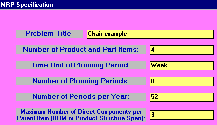
In turns of entering our example problem into the package the screen below is the initial screen we need to set up number of items, time units etc.

The package input for our items is as below

In order to show the make-up (in terms of the parts needed for production)
we have a Bill of Materials (BOM) for the end-product (namely the
chair). Below we show the BOM for the chair.
                       chair
                       |
       +-------------------------------+
       |               |               |
       seat(1)         back(1)         legs(4)
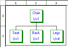
This BOM means that to produce one chair we need:
The Bill of Materials can be thought of as a diagrammatic recipe. Just as in cooking we need a list of ingredients and their quantities to know how to cook something, so here the BOM tells us what we need to make a chair.
The BOM is best thought of as being divided into levels, with the final item (the chair) being at the top level and the items needed to make up a chair being at the second level.
Other examples may have more levels, e.g. if items at the second level are themselves made up from further items. Plainly BOM's are structural information that change relatively infrequently. It is also plain that any mistakes in specifying BOM's could have disastrous consequences on the shop floor - e.g. consider what would happen if we fail to note that a particular part is needed in the production of some item.
In terms of the package we can enter this BOM as below.

This BOM can also be shown graphically by the package, as below.
The tactical information required in MRP relates to:
We deal with each of these in turn below.
Below we give a diagrammatic overview of the situation.
We have specified above structural information about how the items relate to each other (BOM) and item information (e.g. lot size rule); and we will shortly (below) specify tactical information about planned production and inventory in/out/on-hand.
Given all this information then (conceptually at least) we should be able to calculate what we should do, in terms of when to place orders with external suppliers (or internal suppliers) and the size of those orders, so that we never run out of stock of any item i.e. we always achieve the planned production and meet the sales orders.
This process of calculating the orders needed is called a MRP EXPLOSION and produces the materials requirements (hence the name - Materials Requirements Planning).
An important point to note is that MRP is not cost driven i.e. it does not seek to minimise cost (unlike the MPS system used in the package). Instead MRP is stockout driven - that is it will always order sufficient to avoid stockouts (using the lot size rule for each item) and order as late as possible.
We can now specify the tactical information required.
The table below shows the current out-going inventory (predicted or expected sales). For our simple example this is just the forecast demand for chairs.
Time        Quantity
Week 1       150
Week 3        70
Week 5       175
Week 7        90
Week 8        60
We need to produce a detailed production plan for seats, backs and legs to meet this demand. To do this we enter this demand data into the package as below.


Then a detailed production plan can be obtained via an MRP explosion (as will be seen below).
We can however use the MRP package another way - to examine meeting a predetermined production schedule for chairs. Above we have just taken our chair requirements as relating to the total demand. We could however, have entered any numbers there - for example a chair production plan as determined from a cost based master production schedule (MPS). In that case we simply enter the chair figures from the MPS as the chair requirements and the package will produce a detailed production plan for seats, backs and legs to met those requirements.
For the simple example we consider here we shall just take the chair requirements as equal to the demand data.
Note here that the feasibility in terms of production capacity etc of producing the seats, backs and legs in any period to met our chair requirements is not considered in MRP.
This is an important point. MRP typically takes no account of capacity considerations. Such considerations must be taken into account when the MPS is produced.
Note here that our package does not include the capability to take capacity into account. Although we can enter capacity data into the package this is only used for reporting proposes - to see whether we are exceeding production capacities or not. Capacities are not taken into account when the package decides what we need to produce and when.
On-hand inventory is the amount of inventory on-hand at the start of the planning period. For our simple example this is:
Item       On-hand
           inventory
           (units)
chair      260
seat        60
back        40
legs        80
In-coming inventory is the items we expect to receive as a result of buying-in (purchasing) from external suppliers, or items we expect to receive as a result of internal orders placed earlier. For our simple example this is:
Time        Item    Quantity
Week 1      seat    50
Week 1      back    10
This data is entered into the package as below.

Below we show annotated MRP output from the package (after explosion "Explode Materials Requirements") for the example given above for all items.
Chair

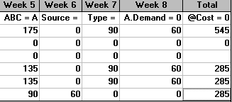
From the last line "Planned Order Release" we see that we need to order 135 chairs in week 3, 90 in week 5 and 60 in week 6. These are as we would expect, since for our simple example we manually calculated when we needed to order chairs to met demand. The benefit of MRP is that the process is automated (hence quicker and less error-prone), and also that we can easily take other items that go to make up a chair (such as seat, back and legs) into account.
In the output above the columns represent different periods and the rows mean:
Seat

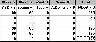
From this output we can see that we are advised to place an order for 25 seats in week 1. This advice should be followed unless there is a good reason for not doing so! You can see why this order occurs, because we have a gross requirement for seats of 135 in week 3, why - because the Planned Order Release for the chair called for 135 chairs in week 3, and we need the seats to be available when we release the order to make the chairs.
Other planned order releases for seats are 90 in week 3 and 60 in week 4.
Back


From this output we can see that we are advised to place an order for 85 backs in week 1. This advice should be followed unless there is a good reason for not doing so! You can see why this order occurs, because we have a gross requirement for backs of 135 in week 3, why - because the Planned Order Release for the chair called for 135 chairs in week 3, and we need the backs available to make the chairs. We already have 40 backs on-hand, another 10 projected to be received in week 1 so we only need to order 135-10-40=85 new backs to have 135 backs available for the chairs in week 3.
Legs

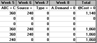
From this output we can see that we are advised to place an order for 460 legs in week 2. This advice should be followed unless there is a good reason for not doing so! You can see why this order occurs, because we have a gross requirement for legs of 540 in week 3, why - because the Planned Order Release for the chair called for 135 chairs in week 3, and we need the legs (4 per chair) available to make the chairs. Since we already have 80 legs on-hand we only need 540-80 = 460 new legs ordered.
Using the package we can get a summary of all actions (planned order releases) as below.

It is often important to conduct sensitivity (what-if) analysis in MRP. Considering the example above, for instance, the only actions we need to take now relate to the orders suggested for the current period. All other actions relate to orders that we may (or may not) place at future points in time. These can be reviewed once the future arrives in the light of new information. Hence the orders suggested for the current period (for seats and backs in this case) are the ones to concentrate on with respect to sensitivity analysis.
So, for example, suppose the demand for the chair is more than expected in week 8. Does this impact upon the actions we must take now or not? If it does then we perhaps need to review the suggested order quantities for seats and backs accordingly.
To illustrate this suppose we change the demand for chairs in week 8 from 60 to 80, i.e. increase it. Changing the package data and re-exploding we get the action (planned order releases) list as

compared with the previous action list of

Here it can be seen that the actions are identical until week 4. At that time we need to begin ordering more items to fulfil the projected increase in demand for chairs.
Extensions
To extend our example suppose that each leg is made up from two components (X and Y). Two units of X and 3 units of Y are needed for one leg and the lead time is 1 week. Then our BOM is:
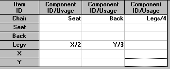
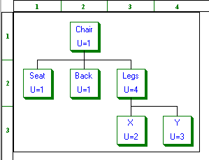
with the item data being:
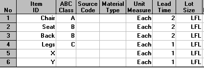
Exploding we get that the action list is:

MRP II is (essentially) MRP but with more added. Typically an MRP II package will include features such as cost information, management reports and easy "what-if" analysis. It may also include capacity requirements planning (essentially try and automatically include capacity restrictions in the planning process).
To confuse things MRP II stands for manufacturing resources planning, signifying that we are concentrating upon the planning of the manufacturing resources (e.g. people, machines, storage), rather than limiting ourselves to the planning of the materials requirements.
As an example of the use of MRP II we have the following:
This company looked at over 40 MRP II packages before choosing Control:Manufacturing from Cincom. The manufacturing operation at their Fernhurst plant is complex with as many as 4,500 finished products being processed from 13,500 different raw materials. Before the days of MRP II stock levels were high and forecasting was hit and miss.
A £1 million MRP II installation has helped bring about some radical operational improvements since it was installed. A good example has been in inventory records and bill of materials accuracy. A BOM administrator was appointed to monitor data accuracy with a regular audit of a dozen BOM's.
In addition, staff had to be trained to a very high detailed level, learning how to structure the BOM's to support customer service objectives, inventory objectives, order entry objectives and costing objectives. Data integrity increased from around 65% to 98% in just six months as a result.
There are many MRP packages available. One example can be seen here.
Just-in-time (JIT) and MRP are two different systems for controlling production. It is often said that:
Really this is an incorrect analysis - MRP is a system based on fulfilling predicted usage in a set time period. This can be seen in the example considered above. We never stocked out.
JIT is a system based on actual usage - parts of the production system are "linked" together via the use of Kanban's as the system runs.
It is this linkage that is the distinguishing difference between MRP and JIT - JIT is a dynamic linked system, MRP is not. This implies that JIT can be used when lead times are short, MRP is more appropriate when lead times are long.
In addition MRP is much better suited for computerised implementation then JIT. Consider, for example, the large number of finished products (4,500) and raw materials (13,500) mentioned in the ICI example considered above. Do you relish the idea of controlling that factory via a JIT system, or would you prefer a computerised MRP system?