OR-Notes are a series of introductory notes on topics that fall under the broad heading of the field of operations research (OR). They were originally used by me in an introductory OR course I give at Imperial College. They are now available for use by any students and teachers interested in OR subject to the following conditions.
A full list of the topics available in OR-Notes can be found here.
The basic function of stock (inventory) is to insulate the production process from changes in the environment as shown below.
Note here that although we refer in this note to manufacturing, other industries also have stock e.g. the stock of money in a bank available to be distributed to customers, the stock of policemen in an area, etc).
One point to note from the above diagram is that most of the activities are a cost - it is only at the final point (sales of finished goods) that we get revenue to set against our costs and hopefully make a profit (= revenue - cost). Hence if we have cost associated with stock we need to deal with that stock in an Effective, Efficient and Economic manner (the 3E's as I tend to term it).
The question then arises: how much stock should we have? It is this simple question that inventory control theory attempts to answer.
There are two extreme answers to this question:
a lot
none/very little
We shall consider the problem of ordering raw material stock but the same basic theory can be applied to the problem of:
The costs that we need to consider so that we can decide the amount of stock to have can be divided into stock holding costs and stock ordering (and receiving) costs as below. Note here that, conventionally, management costs are ignored here.
Note here that a stockout occurs when we have insufficient stock to supply customers. Usually stockouts occur in the order lead time, the time between placing an order and the arrival of that order.
Given a stockout the order may be lost completely or the customer may choose to backorder, i.e. to be prepared to wait until we have sufficient stock to supply their order.
Note here that whilst conceptually we can see that these cost elements are relevant it can often be difficult to arrive at an appropriate numeric figure (e.g. if the stock is stored in a building used for many other purposes, how then shall we decide an appropriate allocation of heating/lighting/security costs).
To see how we can decide the stock level to adopt consider the very simple model below.
In this basic model we have the situation where:
Assume:
Then we need to decide Q, the amount to order each time, often called the batch (or lot) size.
With these assumptions the graph of stock level over time takes the form shown below.
Consider drawing a horizontal line at Q/2 in the above diagram. If you were to draw this line then it is clear that the times when stock exceeds Q/2 are exactly balanced by the times when stock falls below Q/2. In other words we could equivalently regard the above diagram as representing a constant stock level of Q/2 over time.
Hence we have that:
where Q/2 is the average (constant) inventory level
where (R/Q) is the number of orders per year (R used, Q each order)
So total annual cost = ch(Q/2) + co(R/Q)
Total annual cost is the function that we want to minimise by choosing an appropriate value of Q.
Note here that, obviously, there is a purchase cost associated with the R units per year. However this is just a constant as R is fixed so we can ignore it here.
The diagram below illustrates how these two components (annual holding cost and annual order cost) change as Q, the quantity ordered, changes. As Q increases holding cost increases but order cost decreases. Hence the total annual cost curve is as shown below - somewhere on that curve lies a value of Q that corresponds to the minimum total cost.
We can calculate exactly which value of Q corresponds to the minimum total cost by differentiating total cost with respect to Q and equating to zero.
d(total cost)/dQ = ch/2 - coR/Q² = 0 for minimisation
which gives Q² = 2coR/ch
Hence the best value of Q (the amount to order = amount stocked) is given by
and this is known as the Economic Order Quantity (EOQ)
This formula for the EOQ is believed to have been first derived in the early 1900's and so EOQ dates from the beginnings of mass production/assembly line production.
To get the total annual cost associated with the EOQ we have from before that total annual cost = ch(Q/2) + co(R/Q) so putting Q =(2Rco/ch)0.5 into this we get that the total annual cost is given by
ch((2Rco/ch)0.5/2) + co(R/(2Rco/ch)0.5) = (Rcoch/2)0.5 + (Rcoch/2)0.5 = (2Rcoch)0.5
Hence total annual cost is (2Rcoch)0.5 which means that when ordering the optimal (EOQ) quantity we have that total cost is proportional to the square root of any of the factors (R, co and ch) involved. For example, if we were to reduce co by a factor of 4 we would reduce total cost by a factor of 2 (note the EOQ would change as well). This, in fact, is the basis of Just-in-Time (JIT), to reduce (continuously) co and ch so as to drive down total cost.
To return to the issue of management costs being ignored for a moment the basic justification for this is that if we consider the total cost curve shown above, then - assuming we are not operating a policy with a very low Q (JIT) or a very high Q - we could argue that the management costs are effectively fixed for a fairly wide range of Q values. If this is so then such costs would not influence the decision as to what order quantity Q to adopt. Moreover if we wanted to adopt a more quantitative approach we would need some function that captures the relationship between the management costs we incur and our order quantity Q - estimating this function would certainly be a non-trivial task.
A retailer expects to sell about 200 units of a product per year. The storage space taken up in his premises by one unit of this product is costed at £20 per year. If the cost associated with ordering is £35 per order what is the economic order quantity given that interest rates are expected to remain close to 10% per year and the total cost of one unit is £100.
We use the EOQ formula,
EOQ = (2Rco/ch)0.5
Here R=200, co=35 and the holding cost ch is given by
ch = £20 (direct storage cost per unit per year) + £100 x 0.10 (this term the money interest lost if one unit sits in stock for one year)
i.e. ch = £30 per unit per year
Hence EOQ = (2Rco/ch)0.5 = (2 x 200 x 35/30)0.5 = 21.602
But as we must order a whole number of units we have that:
EOQ = 22
We can illustrate this calculation by reference to the diagram below which shows order cost, holding cost and total cost for this example.
With this EOQ we can calculate our total annual cost from the equation
Total annual cost = ch(Q/2) + co(R/Q)
Hence for this example we have that
Total annual cost = (30 x 22/2) + (35 x 200/22) = 330 + 318.2 = £648.2
Note: If we had used the exact Q value given by the EOQ formula (i.e. Q=21.602) we would have had that the two terms relating to annual holding cost and annual order cost would have been exactly equal to each other
i.e. holding cost = order cost at EOQ point (or, referring to the diagram above, the EOQ quantity is at the point associated with the Holding Cost curve and the Order Cost curve intersecting).
i.e. (chQ/2) = (coR/Q) so that Q = (2Rco/ch)0.5
In other words, as in fact might seem natural from the shape of the Holding Cost and Order Cost curves, the optimal order quantity coincides with the order quantity that exactly balances Holding Cost and Ordering Cost.
Note however that this result only applies to certain simple situations. It is not true (in general) that the best order quantity corresponds to the quantity where holding cost and ordering cost are in balance.
We can also solve this problem using the package, the input and output being shown below. Note here that the package can deal with more complicated factors than we have considered in the simple example given above.
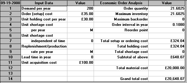
Note the appearance here of the figure of 20,000 relating to material cost. This is calculated from using 200 units a year at a unit cost of £100 each. Strictly, this cost term should have been added to the total annual cost equation (ch(Q/2) + co(R/Q)) we gave above. We neglected it above as it was a constant term for this example and hence did not affect the calculation of the optimal value of Q. However, we will need to remember to include this term below when we come to consider quantity discounts.
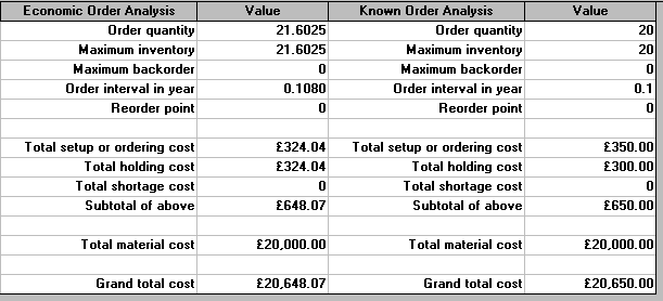
Suppose, for administrative convenience, we ordered 20 and not 22 at each order - what would be our cost penalty for deviating from the EOQ value?
With a Q of 20 we look at the total annual cost
= (chQ/2) + (coR/Q)
= (30 x 20)/2 + (35 x 200/20) = 300 + 350 = £650
Hence the cost penalty for deviating from the EOQ derived value of 22 and ordering 20 at each order is £650 - £648.2 = £1.8
Note that this is, relatively, a very small penalty for deviating from the EOQ value. This is usually the case in inventory problems i.e. the total annual cost curve is flat near the EOQ so there is only a small cost penalty associated with slight deviations from the EOQ value (see the diagram above).
This is an important point. Essentially we should view the EOQ as a ballpark figure. That is it gives us a rough idea as to how many we should be ordering each time. After all our cost figures (such as cost of an order) are likely to be inaccurate. Also it is highly unlikely that we will use items at a constant rate (as the EOQ formula assumes). However, that said, the EOQ model provides a systematic and quantitative way of getting an idea as to how much we should order each time. If we deviate far from this ballpark figure then we will most likely be paying a large cost penalty.
The above cost calculation can also be done using the package - see below.
In order to illustrate extensions to the basic EOQ calculation we will consider the following example:
A company uses 12,000 components a year at a cost of 5 pence each. Order costs have been estimated to be £5 per order and inventory holding cost is estimated at 20% of the cost of a component per year.
Note here that this is the sort of cheap item that is a typical non-JIT item.
Here R=12000, co=5 and as the inventory holding cost is 20% per year the annual holding cost per unit ch = cost per unit x 20% = £0.05 x 0.2 per unit per year = 0.01.
Hence EOQ = (2Rco/ch)0.5 = (2 x 12000 x 5/0.01)0.5 = 3464
The package output for this problem is shown below.
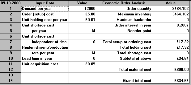
Here we do not have an unrestricted choice of order quantity (as the EOQ formula assumes) but a restricted choice as explained below.
This is an important point - the EOQ calculation gives us a quantity to order, but often people are better at ordering on a time basis e.g. once every month.
In other words we need to move from a quantity basis to a time basis
For example the EOQ quantity of 3464 has an order interval of (3464/12000) = 0.289 years, i.e. we order once every 52(0.289) = 15 weeks. Would you prefer to order once every 15 weeks or every 4 months? Recall here that we saw before that small deviations from the EOQ quantity lead to only small cost changes.
Hence if orders must be made for 1,2,3,4,6 or 12 monthly batches the best order size to use can be determined as follows.
Obviously when we order a batch we need only order sufficient to cover the number of components we are going to use until the next batch is ordered - if we order less than this we will run out of components and if we order more than this we will incur inventory holding costs unnecessarily. Hence for each possible batch size we automatically know the order quantity (e.g. for the 1-monthly batch the order quantity is the number of components used per month = R/12 = 12000/12 = 1000).
As we know the order quantity we can work out the total annual cost of each of the different options and choose the cheapest option.
The total annual cost (with an order quantity of Q) is given by (chQ/2) + (coR/Q) and we have the table below:
Batch size option   Order quantity Q       Total annual cost
Monthly             1000                   65
2-monthly           2000                   40
3-monthly           3000                   35
4-monthly           4000                   35
6-monthly           6000                   40
12-monthly          12000                  65
The least cost option therefore is to choose either the 3-monthly or the 4-monthly batch.
In fact we need not have examined all the options. As we knew that the EOQ was 3464 (associated with the minimum total annual cost) we have that the least cost option must be one of the two options that have order quantities nearest to 3464 (one order quantity above 3464, the other below 3464) i.e. either the 3-monthly (Q=3000) or the 4-monthly (Q=4000) options. This can be seen from the shape of the total annual cost curve shown below. The total annual cost for these two options could then be calculated to find which was the cheapest option.
Order quantity     Cost (per unit)
0-4,999            £0.05
5,000-9,999        £0.05 less 5%
10,000-19,999      £0.05 less 10%
20,000 and above   £0.05 less 15%
For example, were we to order 6000 units we would only pay 0.95(0.05) for each and every one of the 6000 units, i.e. the discount would be given on the entire order.
Here, as mentioned above, we need to remember to add to the total annual cost equation (ch(Q/2) + co(R/Q)) a term relating to R multiplied by the unit cost, as the cost of a unit is now no longer fixed but variable (unit cost = a function f(Q) of the order quantity Q). Hence our total annual cost equation is
ch(Q/2) + co(R/Q) +R[f(Q)]
It is instructive to consider what changes in this equation as we change the order quantity Q. Obviously R and co remain unchanged, equally obviously Q and f(Q) change. So what of ch? Well it can remain constant or it can change. You need to look back to how you calculated ch. If it included money tied up then, as the unit cost f(Q) alters with Q, so too does the money tied up.
The effect of these quantity discounts (breaks in the cost structure) is to create a discontinuous total annual cost curve as shown below with the total annual cost curve for the combined discount structure being composed of parts of the total annual cost curves for each of the discount costs.
The order quantity which provides the lowest overall cost will be the lowest point on the Combined Cost Curve shown in the diagram above. We can precisely calculate this point as it corresponds to:
We merely have to work out the total annual cost for each of these types of points and choose the cheapest.
First the EOQ's:
Discount Cost    ch      EOQ    Inventory   Material   Total
                                cost        cost       cost
0        0.05    0.01    3464   34.64       600        634.64
5%       0.0475  0.0095  3554   Infeasible
10%      0.045   0.009   3651   Infeasible
15%      0.0425  0.0085  3757   Infeasible
Note here that we now include material (purchase) cost in total annual cost.
The effect of the discount is to reduce the cost, and hence ch the inventory holding cost per unit per year - all other terms in the EOQ formula (R and co) remain the same. Of the EOQ's only one, the first, lies within the range covered by the discount rate.
For the breakpoints we have:
Order      Cost    ch       Inventory   Material   Total
quantity                    cost        cost       cost
5,000      0.0475  0.0095   35.75       570        605.75
10,000     0.045   0.009    51          540        591
20,000     0.0425  0.0085   88          510        598
From these figures we can see that the economic order quantity associated with minimum total annual cost is 10,000 with a total annual cost of 591.
Note too here that this situation illustrates the point we made before when we considered the simple EOQ model, namely that it is not true (in general) that the best order quantity corresponds to the quantity where holding cost and ordering cost are in balance. This is because the holding cost associated with Q=10,000 is ch(Q/2) = 0.009(10000/2) = 45, whilst the ordering cost is co(R/Q) = 5(12000/10000) = 6.
This problem can also be solved using the package - the input being shown below. Note that in the package one needs to use Edit Discount Breaks to enter the discount structure.
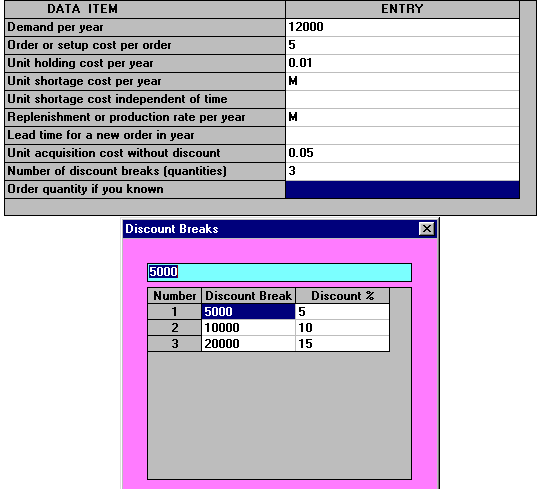
One also needs to use Edit Discount Characteristics. Below we have specified that holding cost is also discounted as the cost of an item changes.
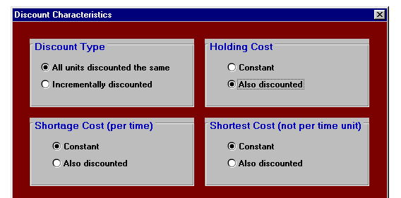
The output from the package is shown below. Notice in that output how the package is considering the same choices (EOQ's and breakpoints) as in our manual calculation above.

Note here the use of discount analysis is not restricted to buyers, it can also be used by a supplier to investigate the likely effects upon the orders he receives of changes in the discount structure. For example if the supplier lowers the order size at which a particular discount is received then how might this effect the orders he receives - will they become bigger/smaller, less frequent/more frequent?
Consider a newsvendor who stands on the street and sells an evening paper, the Evening News. How many copies should he stock?
He sells the paper to his customers for 35 (pence) a copy. He pays his supplier 20 (pence) a copy, but any unsold copies can be returned to the supplier and he gets 10 (pence) back. This is known as a salvage value. Assume that his demand for copies on any day is a Normal distribution of mean 100 and standard deviation 7.
Before we can compute the amount he should order we need to work out his shortage cost per unit - how much does he lose if a customer wants a copy and he does not have a copy available?
As a first analysis he loses his profit (= revenue - cost = 35 - 20 =15) so we can estimate his shortage cost (opportunity cost) as 15 (this ignores any loss of goodwill and any loss of future custom that might result from a shortage).
Giving this information to the package we get:
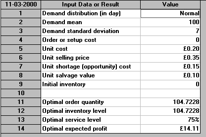
This tells us he should stock 104.7 (say 105) copies of the paper. This service level of 75% means that, on average, he will be able to completely supply his customers on 75 days in every 100, i.e. 3 days out of 4. The remainder of the time (1 day out of 4) he will experience shortages, some customers will not be able to buy a copy from him as he will have run out.
More sophisticated variants of this simple model can be used, for example, to decide how many copies of a magazine to have on a shelf in a newsagent (such as W.H.Smith).
Note that there is an important conceptual difference between this newsvendor problem and the EOQ/discount problems considered above. In those EOQ/discount problems we had a decision problem (how much to order) even though the situation was one of certainty - we knew precisely the rate at which we used items. In the newsvendor problem if we knew for certain how many customers will want a paper each day then the decision problem becomes trivial (order exactly that many). In other words:
There are many extensions to the simple EOQ models we have considered - for example: