OR-Notes are a series of introductory notes on topics that fall under the broad heading of the field of operations research (OR). They were originally used by me in an introductory OR course I give at Imperial College. They are now available for use by any students and teachers interested in OR subject to the following conditions.
A full list of the topics available in OR-Notes can be found here.
The master production schedule (also commonly referred to as the MPS) is effectively the plan that the company has developed for production, staffing, inventory, etc.
It has as input a variety of data, e.g. forecast demand, production costs, inventory costs, etc and as output a production plan detailing amounts to be produced, staffing levels, etc for each of a number of time periods.
This production plan:
The idea of a master production schedule can best be illustrated by means of an example.
In our example we have just a single product being produced.
Production takes place each period (week) either in the normal (regular) production shift or in overtime associated with that shift. There is only one shift (i.e. not operating a two/three shift system - such as with "round-the-clock" working).
Completed items can also be "bought-in" from a subcontractor (at a cost).
We are allowed to hire/fire workers (again at a cost). Backorders are also allowed (recall here that backorders are customer orders that cannot be satisfied in the required period, but the customer allows the order to remain open to be fulfilled in a later period). Lost sales are not allowed.
The diagram below illustrates the situation and the types of factor with which we are dealing graphically.
The data for the example we consider is as below, where we have shown the initial data entry screen from the package.
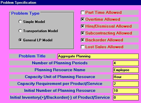
In the above screen we have chosen the "General LP Model". This is the most general of the options allowed by the package. LP stands for linear programming and is a generalised way of modelling decision problems. To ease data entry we have not crossed the "Part Time Allowed" box - if we had then we would have had the option of dealing with part time employees.
We have also not crossed the "Lost Sales Allowed" box - if we had then we would have allowed lost sales. In general a company may allow lost sales because the company finds that customers simply do not backorder - i.e. a lost sale is automatic if the product is not immediately available; or the company is prepared to allow lost sales as it may be better to allow orders to be lost than to allow such orders to become backorders (thereby incurring backorder costs).
The remaining boxes have been crossed and so we can deal with:
In our example above we have just 4 periods (weeks) - this is our time horizon (planning period). We are dealing with employees working hours in each week. Two employee hours are required to produce one unit of each product and the initial number of employees is 10. At the start of the planning period there is no initial inventory (nor are there any backorders).
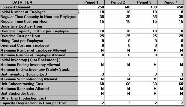
The data for our example entered into the package in the light of the choices made at the initial screen is as below:
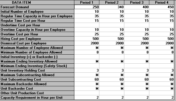
The meaning of each of these lines of data is given below:
Forecast Demand - this is the forecast demand for the product in each of our 4 periods (weeks).
Initial Number of Employee - this is the initial number of employees in each week, here just the 10 employees we have currently.
Regular Time Capacity in Hour per Employee - this is how many regular hours each employee works per week, here 35 hours
Regular Time Cost per Hour - this is the cost per hour of regular time worked, here £15
Undertime Cost per Hour - this is the cost per hour of not using a worker to their full regular capacity, here zero
Overtime Capacity in Hour per Employee - this is the maximum number of hours each employee can work in overtime per week, here 10 hours
Overtime Cost per Hour - this is the cost per hour of overtime, here £25
Hiring Cost per Employee - this is the cost of hiring one employee, here £500
Dismissal Cost per Employee - this is the cost of dismissing (firing) one employee, here £2000
Maximum/Minimum Number of Employee Allowed - here we can set limits on the maximum and minimum number of employees, here M signifies there is no limit on the maximum number and the minimum number is 8. In general there may be an upper limit on the number of employees due to physical capacity constraints.
Initial Inventory (+) or Backorder (-) - the initial inventory available or backorders outstanding, here zero
Maximum/Minimum Ending Inventory - here we can set limits on the maximum and minimum number of product units in stock at the end of each week, here M signifies there is no limit on the maximum number and the minimum number is zero. In general there may be an upper limit because we have a limited space in which to store stock. The minimum number corresponds to safety stock that may be kept in case of unforeseen demand.
Unit Inventory Holding Cost - this is the cost of holding one unit in stock at the end of each period, here £3
Maximum Subcontracting Allowed - this is the maximum number of product units we are allowed to buy in from the external subcontractor, here there is no limit on the amount that may be bought in. In general there may be a limit on the total amount the subcontractor can supply to us each period.
Unit Subcontracting Cost - this is the cost of each unit bought from the external subcontractor, here £60
Maximum Backorder Allowed - this is the maximum number of backorders allowed at the end of each period, here there is no limit on the number of backorders that can be held at the end of each period.
Unit Backorder Cost - this is the cost of each backorder outstanding at the end of each period, here the M signifies that each backorder is very expensive. The effect of M here will be to ensure that (if at all possible) backorders will be avoided.
Other Unit Production Cost - this is the cost of producing one unit of the product that is not already accounted for by employee costs - here zero
Capacity Requirement in Hour per Unit - this is the number of employee hours that are required to produce one unit of the product, here 2 hours
In order to ease understanding of the problem most of the above data items take the same value in each and every period (week). However it would be perfectly possible for them to have different values in each week.
Consider for a moment this example as we have defined it so far. We have a single product, are planning over 4 time periods, have regular time and overtime, can buy from an external subcontractor, and are allowed to hire and fire employees. Some of the decisions we must make are shown below:
                                      Period  1  2  3  4
Amount to produce using regular time          ?  ?  ?  ?
Amount to produce using overtime              ?  ?  ?  ?
Amount to purchase from subcontractor         ?  ?  ?  ?
Number of backorders                          ?  ?  ?  ?
Number to hire                                ?  ?  ?  ?
Number to fire                                ?  ?  ?  ?
You can see from this matrix that there are already 24 decisions which we have to make. For such problems decision models (such as the decision model used within the package) are much better at decision-making than people. Moreover such models can guarantee to make decisions at minimum cost, something people cannot do.
Note here that even the (cheap) package used here is extremely flexible in terms of the situations it can consider.
The solution to the problem is shown below:
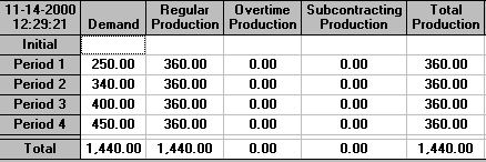
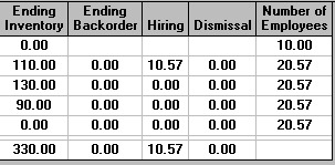
It can be seen that we immediately hire more employees, and that these are employed throughout the planning period of 4 weeks. Note that the number hired is 10.57 - i.e. it includes a fraction of an employee. This often happens in aggregate planning and can usually be ignored (simply round to the nearest appropriate whole number). Reflect that we are producing a plan for production over a 4 week period. It is unlikely that our demand forecasts will be completely accurate and hence this rounding need not concern us unduly.
With 10+10.57 = 20.57 employees working 35 hours a week we have a regular time capacity of 20.57x35 = 720 employee hours (approximately) and at 2 hours per unit produced this corresponds to a regular time production of 360 units - precisely as above, i.e. over the 4 week planning period we are planning to work all of our employees to their full regular time capacity. As can be seen above we are planning no overtime or subcontracting.
Note the build into inventory that occurs in various periods. As inventory costs us money let us be clear about why the above (the minimum cost solution) involves build into inventory. It is to meet future demand. Demand for the product increases over the 4 week planning period (from 250 to 450 units) and the package has determined that the most cost-effective way to ensure that this demand is met is to build into inventory in earlier periods. Note that an alternative strategy to meet this increased demand would be to buy from the subcontractor, were this cheaper the package would have adopted that strategy.
The costs associated with the package solution can be seen below:

The production and employment strategy given above is the minimum cost strategy since the package uses linear programming to calculate a schedule for production and staffing that meets the forecast demand and also satisfies the other constraints that we place upon the problem at minimum cost. It would be impossible to find the minimum cost solution manually - consider the solution shown with an increase in employment and with varying amounts built into inventory - could that ever be produced by a person in the time (fraction of a second) it takes the package to produce it?
We may be interested in a solution that consists of a fixed number of workers (a level strategy). This can be seen below where we have fixed the maximum and minimum number of employees to 10 (the current number) in each and every period.

The solution for this level strategy is shown below.
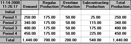
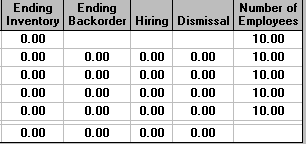

It can be seen that with this solution we use both overtime and subcontracting but do not build into inventory. The total cost of 63,400 is much more than the previous (non-level) strategy which had a total cost of 49475.71
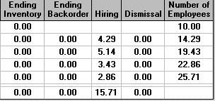
If we change the hire/fire costs to zero and reset the limits on the maximum/minimum number of employees then we will produce a chase strategy (ramp workforce up/down as required). This solution can be seen below.
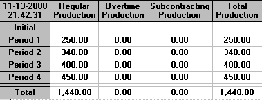

In our original situation considered above, with costs for hiring and firing, we were prohibiting backorders by making them very expensive. Suppose now that backorders cost us £1 per period (week). The effect of this on the solution is shown below.
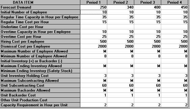
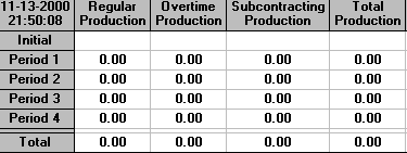
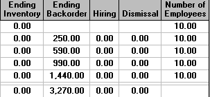
It can be seen that we produce nothing - the cheapest solution is simply to allow backorders to build up over the planning period. This seems silly and for this reason it is usual to insist that there are no backorders outstanding at the end of the planning period. This is an assumption that is, by convention, applied and is a reasonable assumption when planning over a relatively long time period. Moreover unless this is assumed it can happen that the best thing for the company to do over the planning period is simply to allow backorders to build up (as above).
To ensure that there are no backorders outstanding at the end of the planning period we enter a zero for "Maximum Backorders Allowed" in the last period (week 4), as below.
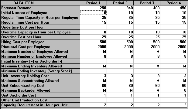
The solution is

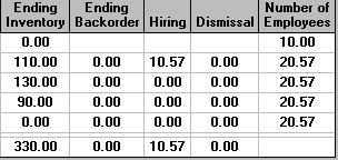
which is effectively the same as the initial solution we considered. However to illustrate that backorders can play a role suppose that we:
then the input is as below:
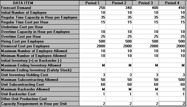
and the output is:

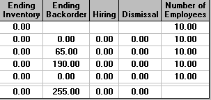

where backorders do occur since production capacity (both regular time and overtime) together with subcontractor capacity is insufficient to met demand in some periods.
In practice we would probably deal with the situation described above on a "rolling horizon" basis in that we would get an initial production plan based on current data and then, after one time period (say), we would update our problem/data and resolve to get a revised production plan. In other words even though we plan for a specific time horizon (here 4 weeks) we would only ever implement the plan for the first week, so that we are always adjusting our 4 week plan to take account of future conditions as our view of the future changes. We illustrate this below.
Period  1 2 3 4 5 6 7       P = plan
        P P P P             D = do (follow) the plan in a period
        D P P P P
          D P P P P
            D P P P P