OR-Notes are a series of introductory notes on topics that fall under the broad heading of the field of operations research (OR). They were originally used by me in an introductory OR course I give at Imperial College. They are now available for use by any students and teachers interested in OR subject to the following conditions.
A full list of the topics available in OR-Notes can be found here.
Stochastic programming, as the name implies, is mathematical (i.e. linear, integer, mixed-integer, nonlinear) programming but with a stochastic element present in the data. By this we mean that:
Stochastic programming therefore deals with situations where we have uncertainty present. We use the abbreviation SP for both stochastic programming and stochastic programs.
For more about stochastic programming than can be found here see here.
Note here that one important thing to realise about the term stochastic programming is that the term is commonly used to cover a number of distinctly different problems. These problems all contain stochastic elements but, as we shall see below, have little else in common.
We consider two distinct stochastic programming problems:
To illustrate one type of stochastic program suppose that we have two six-sided dice. Dice one gives a result a1 when thrown and dice 2 a result a2. Assuming the dice are fair we have discrete probability distributions for a1 and a2 as:
Consider a simple LP with two variables and one constraint:
minimise      5x+6y
subject to:
              a1x + a2y >= 3
              x,y >= 0
What does this LP mean? If a1 and a2 were known numbers we would know exactly what this LP meant, but they are not.
One interpretation could be that we wish the constraint a1x + a2y >= 3 to hold for all possible values of a1 and a2. Then we simply have a deterministic LP with two variables and 36 constraints:
minimise     5x+6y
subject to:
             ix + jy >= 3     i=1,...,6 j=1,...,6
             x,y >= 0
Suppose now that instead of insisting that the constraint a1x + a2y >= 3 holds for all possible values of a1 and a2 we insist that it holds only with a specified probability 1-alpha (where 0 < alpha < 1).
For example alpha=0.05 would mean that we want the constraint a1x + a2y >= 3 to hold with probability 0.95. Note the introduction of probability here, a constraint need not always be true now, rather it need only be true 95% of the time.
Hence the problem is:
minimise     5x+6y
subject to:
             Prob(a1x + a2y >= 3) >= 1-alpha
             x,y >= 0
To summarise this, a1 and a2 are unknown here, we merely have probability distribution information for them. We are required to choose values for x and y such that the objective function is minimised and the probability that the constraint a1x + a2y >= 3 is satisfied is at least 1- alpha.
We might wonder whether this problem is well-defined. To see that it is note that as for each pair of values (a1,a2) we have an associated joint probability (1/36 in this simple case) then:
To see this let us enumerate possibilities for x=0, y=1and alpha=0.05
 a1 a2  Is a10 + a21 >= 3 ?  Probability
  1 1         No               1/36
  2 1         No               1/36
  etc
In this case we already know that x=0 and y=1 is not a feasible solution, since we already have a probability of 2/36 = 0.0555 that the constraint is infeasible. Hence it is impossible for the constraint to be feasible with probability 0.95 (since 1-0.0555 = 0.9445).
Conceptually therefore we could simply enumerate all possible values for x and y and choose those values that minimise 5x+6y.
Hence the problem:
minimise     5x+6y
subject to:
             Prob(a1x + a2y >= 3) >= 1-alpha
             x,y >= 0
is a well-defined problem.
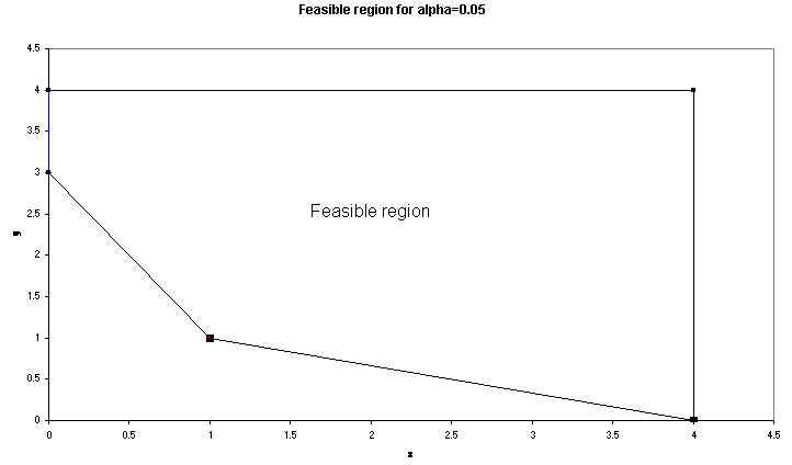
This particular problem (because it contains just two variables) can be easily solved by a simple numeric search procedure. For example for alpha=0.01 the solution is x=3, y=0 and for alpha=0.05 the solution is x=1, y=1.
The feasible region for alpha=0.05 is shown below.

This problem is an example of a stochastic (linear) program with probabilistic constraints. Such problems are also sometimes called chance-constrained linear programs.
Obviously we could easily extend our simple example to:
To solve SP's with probabilistic constraints we transform them into an equivalent deterministic program. Note here however that even if the original SP is linear the equivalent deterministic program may not be. For more on this see here.
SP's with probabilistic constraints as dealt with above are not the only type of stochastic program. Another type that can be defined deals with what are called recourse problems.
In the simplest model of this type we have two stages:
In other words, in the second stage we have recourse to a further degree of flexibility to preserve feasibility (but at a cost). Note particularly here that in this second stage the decisions that we make will be dependent upon the particular realisation of the stochastic elements observed.
To illustrate a simple two-stage recourse model suppose that we have to make a decision about the amount of a product X to produce. Each unit of X that we make costs us £2. X is made to meet demand from customers in the next time period. However demand is stochastic, with a discrete probability distribution: demand = Ds with probability ps (s=1,...,S). Informally we can think of having S scenarios for possible future demand.
Customer demand must be met. We have the flexibility to buy in the product from an external supplier to meet observed customer demand but this costs us £3 per unit (i.e. we have recourse to an additional source of supply if demand exceeds production). How much should we choose to make now before we know what customer demand is?
Below we show one particular example with S=2 and D1=500, p1=0.6; D2=700, p2=0.4. Note here that in this example we have looked forward one period into the future in trying to plan production.
We have to decide how much to produce now before demand is known. If we were to produce 600 (say) then if demand is 500 we are OK, if demand is 700 however we need recourse to an extra 100 units to meet it.
One way to think of this two-stage model is:
You need to be clear about the sequence that applies as you move down the tree in order to formulate the problem correctly.
We proceed as is usual for modelling a problem, by defining variables. Let: x1 >= 0 be the number of units of X to produce now (at the first stage)
As we have S scenarios we associate a scenario subscript with the recourse variables at the second-stage, so let y2s >= 0 be the number of units of X to buy from the external supplier at the second stage in scenario s when the stochastic realisation of the demand is Ds (s=1,...,S).
It is easy to get confused with the subscripts - the order of subscripts is stage,scenario - where the scenario subscript is dropped if the variable is scenario independent.
Then the constraints to ensure that demand is always satisfied are:
x1 + y2s >= Ds s=1,...,S
Note that we must have >= here, the amount x1 we produce may (depending upon the particular demand that occurs) exceed customer demand. If we insisted that x1 + y2s = Ds then as y2s>=0 this would implicitly imply x1<=min[Ds | s=1,...,S].
For the objective function we have a cost 2x1 incurred with certainty and S costs 3y2s, each incurred with probability ps. Note here that, in practice, only one of these S costs will be incurred, once a realisation of the demand occurs. However before that happens we can only consider the probability distribution.
It would seem natural to minimise total expected cost, where total expected cost is:
2x1 + SUM[s=1,...,S]ps(3y2s)
Hence our complete simple SP with (linear) recourse is:
minimise     2x1 + SUM[s=1,...,S]ps(3y2s)
subject to
             x1 + y2s >= Ds       s=1,...,S
             x1 >= 0
             y2s >= 0           s=1,...,S
Note that this is actually a deterministic program. Note too that we could, if we wish, require x1 and y2s to be integer.
Let us be clear about what solving this SP will tell us:
To summarise then, in a two-stage SP with recourse we:
Note here that what made our formulation of the problem simple was the fact that the stochastic element (customer demand) had a discrete distribution. If the stochastic elements have continuous distributions then the mathematical problems associated with formulation and solution become formidable.
We can obtain further insight by solving the above example numerically. Observe that the recourse variables will only play a role if we are short of stock, and we plainly will only buy enough stock to meet demand. Recognising this we can plot out the costs incurred as below.
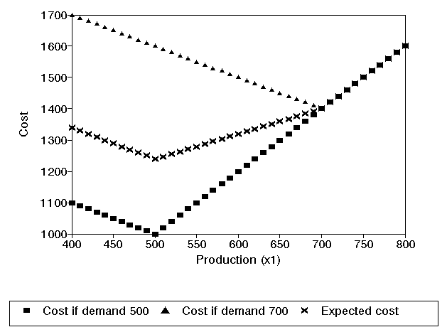
This figure shows the costs that will be incurred under each of the two scenarios, and the expected cost, depending upon our production x1. It is clear from the above figure that the production quantity that minimises expected cost is x1=500.
To check this we can solve this problem using the package. This is shown below where we have solved using the linear programming module in the package and recall here that D1=500, p1=0.6; D2=700, p2=0.4 with ordinary production costing 2 and recourse production costing 3.


Often in SP we look at the worst case - this is the worst possible outcome (given our decision). This is plotted below for our example above.
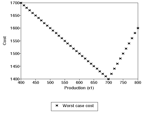
It is clear here that if we are interested in minimising our worst case cost we should produce 700 now.
It is plain that an obvious extension to the above simple two-stage SP with recourse is to have more stages. In such cases it is common that:
To illustrate this we will extend the simple two-stage problem we have considered above to three stages, but using specific numbers rather than a general symbol for the customer demands.
Consider the three-stage binary scenario tree shown below. Note here that in this example we have now looked forward two periods into the future in trying to plan production.
We initially make a decision about how much to produce. At the second stage have two possible realisations of the stochastic demand:
After this realisation we make a decision as to how much to produce to meet demand in the next period (the third-stage).
At the third stage we again (as it is a binary scenario tree) have two possible realisations of the stochastic demand, but these are different depending upon the realisation at the second stage. For example if the realised demand at the second stage was 500 then the possible realisations at the third stage are:
Note here at each level in the scenario tree the appropriate probabilities must sum to one.
This two-level scenario tree actually represents 22=4 possible scenarios of the future:
Scenario Second stage Third stage  Probability
1        500          600          0.6(0.3) = 0.18
2        500          700          0.6(0.7) = 0.42
3        700          900          0.4(0.2) = 0.08
4        700          800          0.4(0.8) = 0.32
Note here that these probabilities add to one (as they must as these 4 scenarios are the only possible futures that we can have).
To summarise then, as we move down the scenario tree (for any scenario) we have the following order of events:
This order naturally extends if we have more than the three stages considered here.
As before, you need to be clear about the sequence that applies as you move down the tree in order to formulate the problem correctly.
In any SP it is important to be clear about the order that pertains as you move through a scenario. In particular you should be clear at each stage about which stochastic elements have been realised and which unrealised.
We can now formulate our three-stage SP. As before let:
x1 >= 0 be the number of units of X to produce now (at
the first stage)
y2s >= 0 be the number of units of X to buy from the external
supplier at the second stage in scenario s (s=1,...,4)
As discussed above, in this three-stage problem we have a decision to make at the second stage, namely the number of units of X to produce at this stage. So let:
x2s >= 0 be the number of units of X to produce at the second stage in scenario s (s=1,...,4)
Note here that (given the order of events we have specified above) this second stage decision is scenario dependent, i.e. dependent upon the observed realisation of the stochastic demand. For example we might well expect to make a different second stage decision if we have observed a customer demand of 700 than if we have observed a customer demand of 500.
We still need our recourse variables for the third-stage so let:
y3s >= 0 be the number of units of X to buy from the external supplier at the third stage in scenario s (s=1,...,4)
For simplicity we will leave the costs (2 for each unit of production, 3 for each unit bought from the external supplier) constant.
The relationship between the order we specified before and the variables is:
Consider the first stage, the constraints to ensure customer demand is satisfied are:
x1 + y2s >= 500    (s=1,2)
x1 + y2s >= 700    (s=3,4)
Now at the second stage we will have units left over (i.e. inventory) to help meet future demand. This inventory level will be:
x1 + y2s - 500    (s=1,2)
x1 + y2s - 700    (s=3,4)
To ensure that demand is met in the third stage we have: inventory + amount produced + amount bought externally >= demand
x1 + y2s - 500 + x2s + y3s >= 600   (s=1)
x1 + y2s - 500 + x2s + y3s >= 700   (s=2)
x1 + y2s - 700 + x2s + y3s >= 900   (s=3)
x1 + y2s - 700 + x2s + y3s >= 800   (s=4)
Whilst these constraints might seem to capture all of the problem in fact there are further constraints that (logically) we need to add.
Consider the recourse variables y2s for s=1 and s=2. These are the amounts bought externally in scenarios 1 and 2 at the second stage. But how can we distinguish between scenario 1 and scenario 2 at the second stage? Both of these scenarios have a common history up to and including the second stage (a decision x1 at the first stage and an observed realisation of the demand at the second stage of 500). It is not until we have a realisation of demand at the third stage that scenarios 1 and 2 differ.
It would seem logical therefore that y21 and y22 must be equal, simply put we cannot have different recourse variables because we cannot distinguish between these scenarios. We can ensure y21 and y22 are equal by adding the constraint y21=y22 to the problem.
In SP constraints which enforce such conditions are called nonanticipativity constraints, implying we cannot anticipate the future.
As the above example has shown, scenarios with a common history must (logically) have the same set of decisions so that we have the complete set of nonanticipativity constraints as:
scenarios 1 and 2, second stage:
     y21=y22
     x21=x22
scenarios 3 and 4, second stage:
     y23=y24
     x23=x24
Note here that this is a key point - scenarios with a common history must have the same set of decisions - and must always be taken into account when formulating a scenario based decision problem.
We can now formulate our objective function. We have just one cost incurred with certainty, namely 2x1, all other costs are probabilistic. The easiest way to summarise these costs is to look at each scenario in turn:
Scenario  Probability  Cost
1         0.18         2x21 + 3y21 + 3y31
2         0.42         2x22 + 3y22 + 3y32
3         0.08         2x23 + 3y23 + 3y33
4         0.32         2x24 + 3y24 + 3y34
Weighting each scenario cost by the associated scenario probability will give the expected cost. Hence we have the objective (minimise total expected cost) as:
minimise
2x1 + 0.18(2x21 + 3y21 + 3y31) + 0.42(2x22 + 3y22 + 3y32)
    + 0.08(2x23 + 3y23 + 3y33) + 0.32(2x24 + 3y24 + 3y34)
This completes our formulation of this particular three- stage stochastic program and for completeness we give the complete formulation below.
minimise
2x1 + 0.18(2x21 + 3y21 + 3y31) + 0.42(2x22 + 3y22 + 3y32)
    + 0.08(2x23 + 3y23 + 3y33) + 0.32(2x24 + 3y24 + 3y34)
subject to
x1 + y2s >= 500    (s=1,2)
x1 + y2s >= 700    (s=3,4)
x1 + y2s - 500 + x2s + y3s >= 600   (s=1)
x1 + y2s - 500 + x2s + y3s >= 700   (s=2)
x1 + y2s - 700 + x2s + y3s >= 900   (s=3)
x1 + y2s - 700 + x2s + y3s >= 800   (s=4)
y21=y22
x21=x22
y23=y24
x23=x24
all variables >=0
We can solve this problem using the package. This is shown below where (as before) we have solved using the linear programming module in the package.
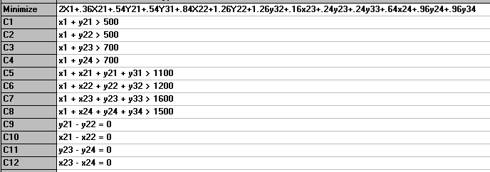
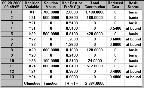
It can be seen that we choose to produce 700 now.
Note here that although, conventionally, the multi-stage stochastic program with recourse is formulated so as to minimise total expected cost other objectives are equally possible.
For example, as we know the total cost associated with each scenario, and the scenarios are the set of all possible futures, we might wish to minimise the maximum cost we would ever have to pay (minimise the maximum scenario cost). This can be formulated by introducing a variable Z and adding to the above formulation:
Z >= 2x1 + (2x21 + 3y21 + 3y31)   scenario 1
Z >= 2x1 + (2x22 + 3y22 + 3y32)   scenario 2
Z >= 2x1 + (2x23 + 3y23 + 3y33)   scenario 3
Z >= 2x1 + (2x24 + 3y24 + 3y34)   scenario 4
The objective function would then become minimise Z
Note that if we formulate the problem this way we do not use the associated scenario probabilities. This may be appropriate if we are very unsure of these probabilities and are reluctant to include them in the standard objective of minimise total expected cost.
This problem is solved below.

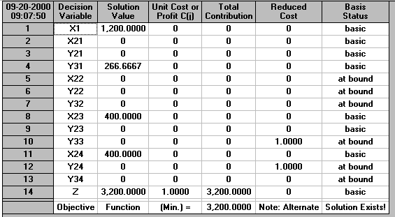
Here we produce 1200 now.
Note too here that whilst this minimise Z objective will ensure that we minimise the maximum scenario cost we need to be aware that with scenarios that cost less than this maximum cost we may have flexibility about variable values. Hence if Z* is the minimum value of Z from this formulation it is appropriate to then solve a further program:
minimise: total scenario cost
subject to: Z <= Z* and the same constraints as above
i.e. minimise
4(2x1) + (2x21 + 3y21 + 3y31) + (2x22 + 3y22 + 3y32)
       + (2x23 + 3y23 + 3y33) + (2x24 + 3y24 + 3y34)
subject to: Z <= Z* and the same constraints as above
This will enable us to obtain variable values that still respect our overall minimum with respect to the maximum scenario cost but which also minimise (total) cost over all scenarios. Note here that this objective effectively gives equal weight to each of the scenarios. If we wished we could incorporate a more explicit probability based weighting here. In fact, if you were wondering why y31 above had such a strange value (266.6667) this is due to the fact that scenario 1 is not important in terms of the worst case so any value for y31 that satisfies the appropriate scenario 1 constraint will do.
The solution to this problem is shown below.
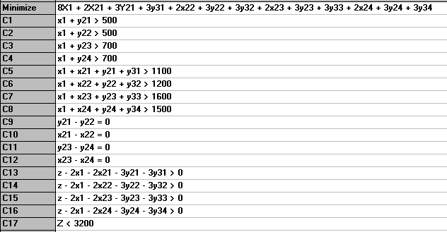
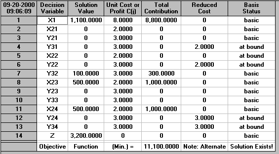
Observe that our stochastic program is actually a deterministic program (in fact a linear program in this particular case). Although the original problem had stochastic elements the use of scenarios to explicitly represent the set of all possible futures has enabled us to formulate the problem deterministically.
With regard to the computational difficulty of solving this (deterministic) stochastic program note that the nonanticipativity constraints can be eliminated by algebraic substitution for variables, this reduces the total number of constraints and variables in the problem.
The real computational difficulty arises due to the number of scenarios that can often appear. Observe that we essentially need a complete set of variables/constraints for each possible scenario. Although as noted above the nonanticipativity constraints reduce the number of distinct variables/constraints the size of the deterministic program increases rapidly with the number of scenarios.
Scenario generation is also a problem in stochastic programming. For example consider our simple problem above where we had three stages corresponding to 2 realisations of demand - that led to 4=22 scenarios - if we have T time periods (realisations of demand) then we will need 2T scenarios (assuming a binary scenario tree as above). The demand that occurs at each stage of these scenarios is meant to be a realistic one - not a randomly generated number - so somehow we must realistically produce demand figures for a large number of possible futures. This is not a trivial task.
Probably the predominant use currently of multi-stage SP's with recourse is in the field of quantitative finance. For example the modelling of an investment portfolio so as to meet random liabilities.
Insurance companies are a good example of such problems. An insurance company receives money in premiums which it can invest in various assets. The investment returns from these assets may be stochastic or deterministic (depending upon the asset). Plainly the insurance claims that the company receives will be stochastic (e.g. in buildings insurance a bad winter will increase the claims for storm damage). Recourse variables would represent the liquidation (selling) of assets to meet liabilities. How then should such a company structure its investment decisions over time so as to use its assets wisely and to meet its liabilities.
Other areas where multi-stage SP's are used include: