
OR-Notes are a series of introductory notes on topics that fall under the broad heading of the field of operations research (OR). They were originally used by me in an introductory OR course I give at Imperial College. They are now available for use by any students and teachers interested in OR subject to the following conditions.
A full list of the topics available in OR-Notes can be found here.
As a manufacturer we are interested in the quality of the product that we produce. As a consumer we are interested in the quality of the product that we buy. Quality often means different things to different people but can generally be regarded as meaning that the product meets certain targets. For a lightbulb quality might mean that it works when we buy it, whilst for a packet of cornflakes quality might mean that we have over a certain minimum amount of cornflakes in the packet. We will consider some ways of measuring the quality of a product and detecting quality changes - both features of a quality control process.
Complete, or 100%, inspection involves inspecting each item that is produced to see if it meets the desired quality level. This might seem to be the best procedure to meet quality targets but in fact it has a number of drawbacks:
Generally 100% inspection is operated for items where the consequences of letting a defective item through could be quite severe e.g. for avionic systems.
If we decide not to operate 100% inspection, for whatever reason, then the alternative is to take a sample of a certain size from a batch (sometimes called lot) of items and operate 100% inspection on the sample. From the results of the sample we decide whether to:
Typically if the proportion of defective items in the sample is below a certain level then we accept the batch - else we reject it. This type of scheme is known as acceptance sampling.
Note here that in all the situations we consider we assume that inspection is 100% effective (i.e. that there are no errors of judgement on the part of the quality inspector, either in classifying a good item as defective or in classifying a defective item as good).
Note too that we can never be absolutely certain about the quality of the batch based on the quality of the sample. For example a random sample of size 50 from a batch of size 500 might have all 50 items OK. It could be (although this seems unlikely) that the remaining 450 items are all defective.
Because we can never be absolutely certain probabilities play a key role in quality control.
Conceptually we can think of an acceptance sampling scheme as a filter between the company (the producer of the batch) and the outside world (the customer or consumer of the batch). Batches come to the filter, samples of a certain size are taken from the batch and the batch is either passed through the filter to the outside world, or it is rejected. It may help to picture this as below:
   The company (producer)

-------------------------------- filter (acceptance sampling scheme)

   The outside world (consumer)
In developing an acceptance sampling scheme we make two statements that we would like our scheme to satisfy: The first of these statements is:
p1 is known as the acceptable quality level (AQL) and alpha is known as the producer's risk. For example suppose alpha = 0.05 and p1 = 0.08. Then putting these values into the above statement we are saying
Suppose for a moment that all batches had a proportion of defectives exactly equal to 0.08. Then our acceptance sampling scheme (whatever it is - and that is still to be decided) should reject 5% of these batches and accept 95%. In other words 95% of such batches would be passed to the consumer. As the vast majority of such batches are passed to the consumer it is clear why 0.08 (p1) is known as the acceptable quality level (AQL). Moreover as 5% (alpha) of the batches are not passed on, but are of an acceptable quality, it is clear why alpha is known as the producer's risk.
The second of the statements we need to define an acceptance sampling scheme is:
p2 is known as the rejectable quality level (RQL) or the lot tolerance proportion defective (LTPD) and beta as the consumer's risk. For example suppose beta = 0.10 and p2 = 0.16. Then putting these values into the above statement we are saying
Suppose for a moment that all batches had a proportion of defectives exactly equal to 0.16. Then our acceptance sampling scheme (whatever it is - and that is still to be decided) sould reject 90% of these batches and accept 10%. In other words 90% of such batches would not be passed to the consumer. As the vast majority of such batches are not passed to the consumer it is clear why 0.16 (p2) is known as the rejectable quality level (RQL). Moreover as 10% (beta) of the batches are passed on, but are of a rejectable quality, it is clear why beta is known as the consumer's risk.
Several different types of general sampling schemes are commonly available (to meet the requirements of our two statements above) and include:
The choice for the producer comes down to deciding which of the available sampling schemes would be best (in terms of cost, administrative convenience, etc) to operate. We shall examine each of these schemes in turn.
Note here however that acceptance sampling is intimately connected with hypothesis testing in statistics. Essentially we are conducting the hypothesis test
H0: batch of an acceptable quality versus H1: batch of a rejectable quality
and we accept or reject H0 based on the evidence from the sample.
In this scheme we take a single sample (of size to be determined) from a batch and accept the batch provided the number of defectives found in the sample falls below a certain number (the acceptance number).
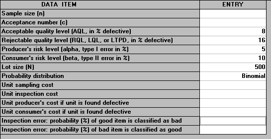
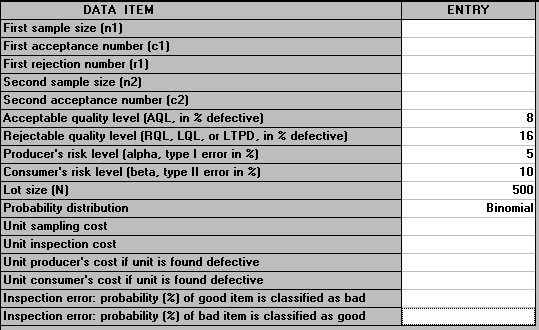
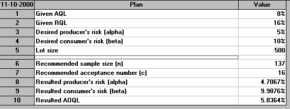
For a problem where we desire the producer's risk alpha to be 0.05 at an associated defective level (p1) of 0.08 and the consumer's risk beta to be 0.10 at an associated defective level (p2) of 0.16, what is the sample size and acceptance number if the lot (batch) size is 500?
Hence we have:
alpha = 0.05 and p1 = AQL = 0.08
beta = 0.10 and p2 = LTPD = RQL = 0.16
Lot size N = 500
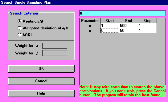
We can now solve this problem using the package. The input is shown below.
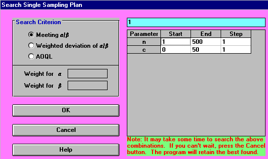
By using "Search Sampling Plans" as below the package will examine all values for n (the sample size) and c (the acceptance number) so as to find a single sampling scheme that best meets the specified values of alpha and beta with appropriate p1 and p2 values.
The output is shown below.
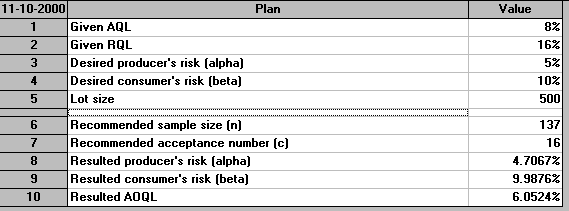
From this output we see that we should take a (random) sample of size 137 from the batch. If the number of defective items found is <= the acceptance number (16 in this case) then we accept the batch, otherwise we reject the batch. With this sampling plan the actual (resulting) producer's risk is 4.7067% and the actual (resulting) consumer's risk is 9.9876%. These numbers are not exactly what we specified (which were 5% and 10% respectively) but are as close as we can get given that we must sample a whole number of items from the batch.
As mentioned above conceptually we can think of the acceptance sampling scheme as a filter between the company and the outside world. Batches come to the filter, samples of a certain size are taken from the batch and if there are less than a certain number of defectives in the sample the batch is passed through the filter, otherwise it is rejected.
Suppose now that we were to send to this filter identical batches, i.e. all with the same number of defectives (say 70 defectives in the entire batch of size 500). Some of these batches would be passed by the filter and some would be rejected (depending on whether we happened, purely by chance, to take more or less defective items in the sample associated with each batch).
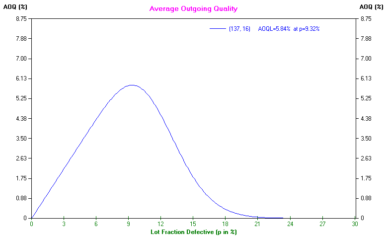
Given this situation it is useful to think of the average outgoing quality (AOQ), namely the average quality of the batches that pass the filter when the filter is presented with identical batches with the same proportion of defective items.
By examining all possible values for the actual proportion of defectives it is possible for the package to work out the average outgoing quality. All values of AOQ against proportion of defectives have been plotted below.
At the left-hand side of the curve below the proportion of defectives in the batches being produced is low, so these batches are accepted and hence the proportion of defectives in the out-going batches is also low. By contrast at the right-hand side of the curve below the proportion of defectives in the batches being produced is high, so these batches will be rejected by the sampling scheme. As no batches will be passed the proportion of defective items in outgoing batches is effectively zero.
Between these two extremes you will see that the AOQ reaches a limit and then declines. This limit is called the average outgoing quality limit (AOQL). It is the maximum (worse) value the average outgoing quality (AOQ) can be under the specific sampling plan suggested, irrespective of how bad the batches the company produces are!
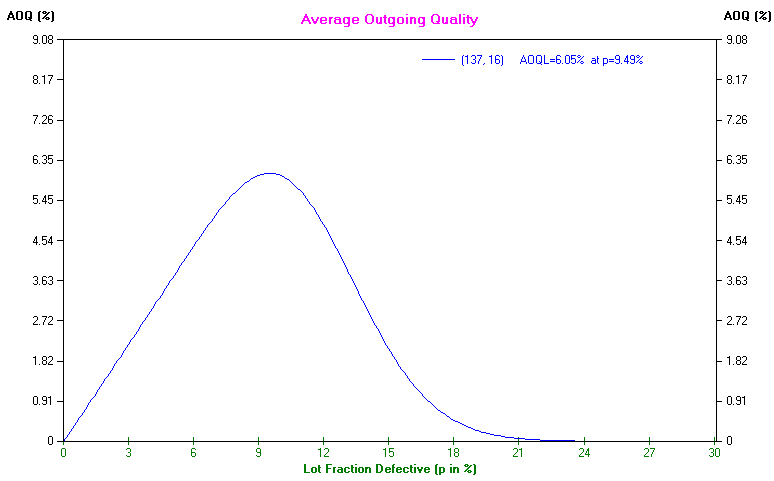
Hence given the above sampling plan (sample size 137, acceptance number 16) then from the package output given above we have that if we do not replace any defective items (found by sampling) in accepted batches the AOQL is 6.05%, i.e. on average at most 6.05% of the items in an outgoing batch will be defective - see the AOQ graph above.
This is an obvious extension of the single sample scheme where we first take a small sample and if this is mainly OK (defective) then the batch is accepted (rejected), otherwise a further sample is taken to decide the fate of the batch.
This scheme allows us to save money, time, effort, etc by not having to go and undertake the same inspection on batches that are mainly OK as we would in the single sample case (if the batch is OK we will be accepting with a smaller sample), and hopefully most of the batches that we test are mainly OK.
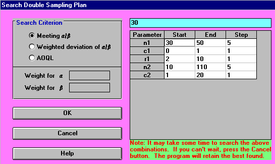
For the problem considered above what would be an appropriate double sampling plan?
Again we can solve the problem using the package with the input being shown below.
The parameter values for searching on (values for n1,c1,r1,n2,c2 below) have been specifically chosen by me for this example so as to give a good result in a relatively short amount of time. Even the restricted values given there involve examining 5 values for n1, 2 values for c1, 9 values for r1, 21 values for n2 and 20 values for c2, so 5x2x9x21x20=37800 distinct combinations to consider. In real life one might have to examine many combinations of parameter values, requiring quite a long time.
The output for the problem is shown below. Again the package solves the problem by finding values for acceptance/rejection numbers and sample sizes so as to best met the specified values of alpha and beta with appropriate p1 and p2 values.
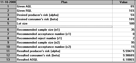
Here the first sample is of size 35 and has an associated acceptance number of zero, i.e. if we get no defective items in this sample then we accept the batch. The reject number associated with this first sample is 2. So if we get 2 or more defectives in this first sample we immediately reject the batch. Otherwise we go on to take a second sample. This second sample is of size 95 and has an associated acceptance number of 15. This means that if the number of defective items from BOTH samples is 15 or less then we accept the batch, else we reject it.
Summarising here we:
An extension of double sampling is multiple sampling whereby we take a number (> 2) of small samples. The idea here is that after each sample we decide to:
This idea of multiple sampling leads naturally to the concept of sequential sampling.
In a sequential sampling scheme we keep testing items from the batch and after each item is inspected we make a decision to either accept or reject the batch, or to continue sampling. The distinction from multiple sampling lies in the fact that in multiple sampling we prespecify the maximum number of samples we will take. With sequential sampling we (potentially) could end up conducting 100% inspection on the entire batch. Contrast this with double sampling above where we could, at most, take two samples - typically both samples comprising less than the entire batch.
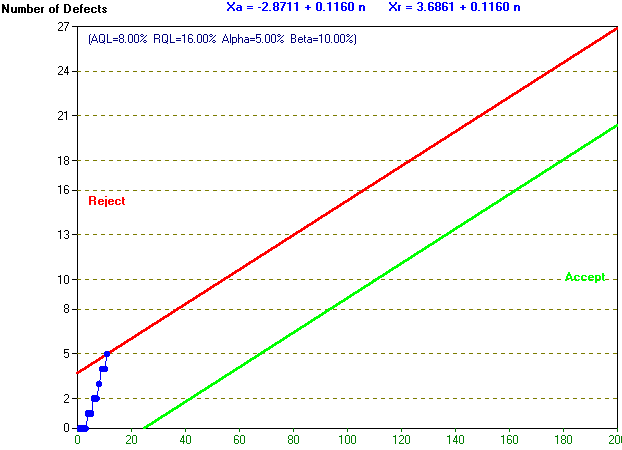
Graphically this can be shown below where the cumulative sample size is n and the cumulative number of defects is X.
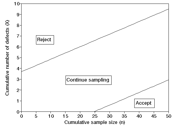
The graph above is divided into three decision regions by the two lines shown there:
For the problem we considered before we can calculate the sequential sampling plan using the package. The output is shown below
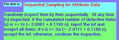
From this we can see that (for this example) the upper line is given by the equation:
X = 0.1160n + 3.6861
and the lower line is given by the equation:
X = 0.1160n - 2.8711
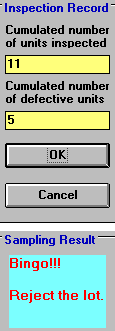
This implies that for n = 10 (for example) we continue sampling if the cumulative number of defective items lies between (1.160 + 3.6861) and (1.160 - 2.8711) = (4.85 to -1.71 (approximately)). Hence at that stage we will reject the batch if 5 or more defective items have been found but the sample is still too small for us to be prepared to accept the batch.
This behaviour is illustrated below where, from the package, we have used the What-If analysis to simulate the inspection process where at a sample size of 10 we have 4 defectives and hence need to continue sampling but at a sample size of 11 we have had 5 defective items and can reject the batch.
Under a scheme of this kind, all rejected batches are subjected to 100% inspection of the batch and rectification - that is all the defective items in the batch are replaced with items that are OK. The consumer will receive two types of batches:
For the example we had before a single sample rectifying plan is as below.
It will be seen that although the sample size and acceptance numbers are the same in this case as the single sample case considered above the AOQL is less than before (as we might expect).
Note here however that the right-hand end of the above curve is fundamentally different in nature from the AOQ curve we saw before for single sampling. In the curve we saw previously the proportion of defectives in out-going batches was zero because no batches were out-going, all batches being rejected by the sampling scheme. In the curve above for a rectifying scheme the proportion of defectives in an out-going batch is low at the right-hand end of the curve since the batch will have been rectified (i.e. subject to 100% inspection and all defective items replaced by good items).
Be aware that confusion exists in the literature, some authors implicitly present AOQ curves as if rectification takes place, some do not.
Standard quality control schemes are easily available to assist in choosing an appropriate scheme. Typically these are based on government defence industry schemes and are more complicated than the simple schemes we have considered above although the underlying principles are the same. The main areas of additional complexity are:
All the sampling schemes we have considered so far have dealt with sampling by attributes - that is an item always had the attribute "defective" or not. If the quality characteristic is a continuous variable (e.g. the length of a manufactured object) then we need a different type of sampling scheme - namely sampling by variables.
In such schemes we often have a desired quality target T and we are looking at the variation in the continuous quality variable from T. We shall examine just one technique - control charts. More about control charts can be found here.
Control charts, or Shewhart charts are used to detect changes in the quality q of the manufactured product. Suppose that the desired quality target is T then we plot the measured quality q against time on a graph as shown below, where the warning and action lines are centred around the target T and indicate that the quality is deviating from the desired level T. Note that in some cases we may be interested in deviations in one direction only.
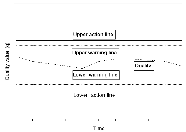
Where the warning and action lines are set determines the frequency with which you interfere with the production process to get the quality back on target. If these lines are far away from T then you never interfere (even when the quality is way off target), but if they are too close to T then you are interfering all the time (even when the quality has not actually gone off target but a deviation from T has been observed because of sampling errors).
A useful interpretation of the warning/action lines about T is that they represent limits on the natural variation of the quality variable. Any observations outside these lines are probably due to unnatural variation and are deserving of closer investigation.
Often the warning lines are set at T ± 2sigmaT and the action lines at T ± 3sigmaT where sigmaT is the standard deviation of the quality when the underlying average is actually T. This means that there is a probability of approximately 95% of remaining within the warning lines (when the process is actually on target) and a probability of approximately 99.7% of remaining within the action lines (when the process is actually on target). Note that this means that observations outside these lines are probably due to unnatural variation, however we can never be sure of this - there is a small chance that such observations are simply extreme natural variation.
There are two approaches for setting T and sigmaT. One approach is to specify them explicitly, i.e. assign them values, the other approach is to deduce them from sample observations of the quality variable. The second of these two approaches (deduce from sample observations) is the approach we shall take in the example below.
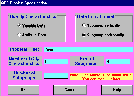
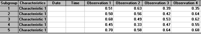
In the data below we show the results for the diameter (in inches) of a pipe for each of five samples (four observations per sample). If, historically, the process has been on target, is it still on target?
Sample      Observations
number      1     2     3     4
1           0.51  0.63  0.39  0.35
2           0.50  0.56  0.42  0.64
3           0.68  0.49  0.53  0.62
4           0.45  0.33  0.47  0.55
5           0.70  0.58  0.64  0.68
This problem can be solved using the package. (The input is shown below).
To determine whether the process is in control or not we first need to set up the control limits, as below for example.
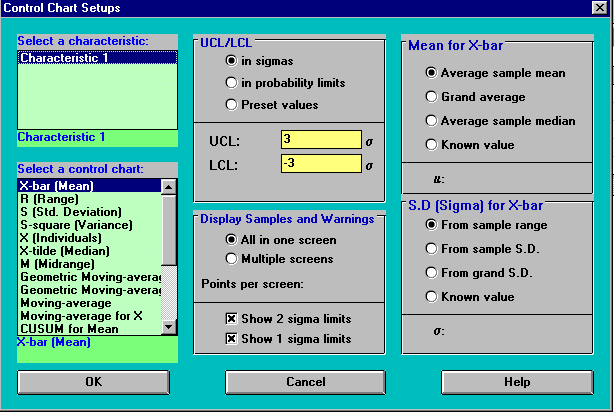
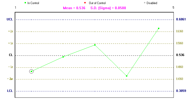
Above we have set a 3 sigma limit, i.e. ± 3sigmaT. Below we show the process average (X-bar chart), this is a graph of the average for the observations in each sample together with the associated upper and lower confidence lines (UCL and LCL below). One peculiarity of the package is that it assumes that the current (latest) sample is sample number 1 (subgroup number 1 in package terminology). In reality it is much easier to read control charts as if time is flowing from left to right.
Below we show the range chart (R chart), this is a graph of the range for the observations in each sample together with the associated upper and lower confidence lines.
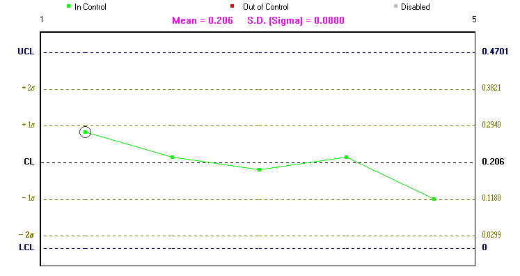
Note here that it is important to look at both the X-bar chart, the process average, and the R chart, the process range. This is because whilst one of these charts may be within the associated upper and lower confidence lines the other may not be (as occurs above, where we have one observation in the X-bar chart outside the 2sigmaT limit).
The logic behind these charts is that normally we would expect all observations to lie between the lower and upper confidence lines. If we get an observation lying outside these lines then this could be due to chance (remember there is a small chance (about 0.3%) of deviating outside the upper and lower confidence lines when the process is on target) or could be indicative of the process being off target.
In practice what might happen from the graphs shown above is that once we detect deviations outside the upper and lower confidence lines we would step up the frequency of sampling. This would enable us to see if these deviations are by chance.
Choosing a quality control scheme nowadays requires the cost of inspection to be balanced against the ease of administering the scheme. Software is available to help decide sample sizes and acceptance numbers in the case of sampling by attributes. Any situation where inspection is not 100% effective means that care should be taken in blindly applying the results from such software.