OR-Notes are a series of introductory notes on topics that fall under the broad heading of the field of operations research (OR). They were originally used by me in an introductory OR course I give at Imperial College. They are now available for use by any students and teachers interested in OR subject to the following conditions.
A full list of the topics available in OR-Notes can be found here.
Graph theory deals with problems that have a graph (or network) structure. In this context a graph (or network as many people use the terms interchangeable) consists of:
An example graph is shown below.
Graph theory is used in dealing with problems which have a fairly natural graph/network structure, for example:
Note here that the minimum cost network flow problem (also dealt with in this course) is an example of a problem with a graph/network structure.
Some of you may be reading this document via the Web. That is also a graph, with each document (file) being a node and each hypertext link (the thing you click on to go elsewhere) an arc.
Graph theory has a relatively long history in classical mathematics. In 1736 Euler solved the problem of whether, given the map below of the city of Konigsberg in Germany, someone could make a complete tour, crossing over all 7 bridges over the river Pregel, and return to their starting point without crossing any bridge more than once.
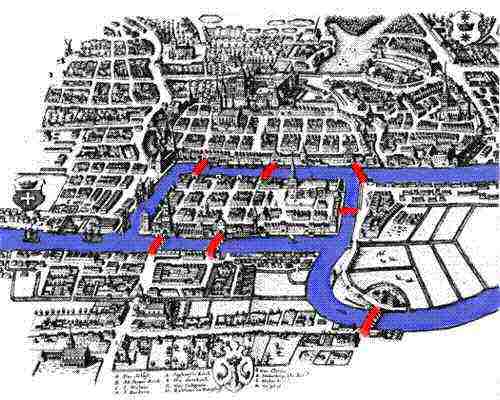
(map courtesy of The MacTutor History of Mathematics Archive).
See if you can reach the same conclusion as Euler did. The picture below shows the city, but simplified so that just the river and bridges are shown - do you think that someone could make a complete tour, crossing over all 7 bridges over the river, and return to their starting point without crossing any bridge more than once.

The area of algorithmic graph theory (algorithms to solve graph theory problems) came to prominence in the mid 1970's with the work of Nicos Christofides (Imperial College Management School) and has become more fashionable/well-known since then.
In this note we consider two graph theory problems relating to spanning trees and shortest paths in detail and outline the multinational tax planning problem. More about graph theory can be found here.
Consider the following problem. In the diagram shown below we have four wells in an offshore oilfield (nodes 1 to 4 below) and an on-shore terminal (node 5 below). The four wells in this field must be connected together via a pipeline network to the on-shore terminal.
The various pipelines that can be constructed are shown as links in the diagram below and the cost of each pipeline is given next to each link. What pipelines would you recommend be built?
It is clear that this particular problem is a specific example of a more general problem - namely given a graph (such as that shown above) which links would we use so that:
This problem is called the shortest spanning tree (SST) problem. Note here that the phrase "minimal spanning tree" (MST) is also often used instead of the phrase "shortest spanning tree" (SST).
For example, in the diagram above, one possible structure connecting all the points together would consist of the links 1-2, 2-3, 3-4, 4-5 and 5-1, but there are other structures where the total cost of the links used is smaller than in this structure (e.g. drop any link in the circle (cycle) 1-2-3-4-5-1 formed above).
Points to note :
We consider below the Kruskal algorithm for finding the shortest spanning tree of a graph.
The algorithm is:
"For a graph with n nodes keep adding the shortest (least cost) link - avoiding the creation of circuits - until (n-1) links have been added"
Note here that the Kruskal algorithm only applies to graphs in which all the links are undirected.
For the graph shown above, applying the Kruskal algorithm and starting with the shortest (least cost) link, we have:
Link   Cost   Decision
1-5    2      add to tree
1-2    3      add to tree
1-4    3      add to tree
5-4    4      reject as forms circuit 1-5-4-1
5-2    5      reject as forms circuit 1-5-2-1
2-3    6      add to tree
Stop as 4 links have been added and these are all
we need for the SST of a graph with 5 nodes.
Hence the SST of the graph shown above consists of the links 1-5, 1-2, 1-4 and 2-3 (total cost 14) and is as shown below.
Note here that in applying the Kruskal algorithm we often encounter the situation in which two (or more) links have the same cost (e.g. consider links 1-2 and 1-4 in the above example). In such a case the order in which these (equal cost) links are considered does not matter [different SST's may result depending upon the order chosen but they will all have the same total cost and this cost will be the minimum that can be achieved].
The problem shown above was also solved using the package, the input being shown below.
The output is shown below.
The principal limitation of the pipeline network shown is (in practical terms) that we have ignored the fact that some pipelines carry more oil than others and this means that they must therefore be of larger diameter and hence more expensive (per unit length).
We therefore have the situation that the cost of a pipeline depends upon the amount of oil it must carry - but we do not know how much oil any particular pipeline is carrying until we have decided the entire pipeline network.
Iterative application of SST calculations provides one way of solving such practical pipeline design problems. Typically we first set a cost for each pipeline, then
Other difficulties include:
A pioneering application of SST models to pipeline network design (due to Frank and Frisch) occurred in the early 1960's in the design of a gas pipeline network in the Gulf of Mexico. Savings resulted of the order of tens of millions of dollars. This illustrates how, in OR, nice neat theoretical problems (like the SST) can be used as building blocks to solve complex practical problems.
The above problem can be considered as a network design problem. Such problems typically involve a number of distinct points (nodes) and connections between pairs of nodes (links) and the problem is to design a suitable network to connect together a number of the nodes at minimum cost and which satisfies a number of criteria. For example we may want a minimum cost network which still functions after a failure in any one of the links.
Such problems are increasingly important nowadays, in particular in the telecommunications industry. In the simplest case the nodes are given, each possible link has a cost associated with its use and the problem is which links should be used so as to minimise total cost whilst ensuring that the network is connected. This problem is precisely the SST problem dealt with above.
Other factors that can occur here are:
More generally we can distinguish between vertex connectivity and edge connectivity:
where by disconnect we mean that the graph remaining after removal is separated into two (or more) pieces.
For example the SST derived above has vertex connectivity 1 and edge connectivity 1.
For the pipeline problem considered above (shown again below):
The answer to the last question of what is the network that is least vunerable to link (edge) failure, i.e. the network that maximises K edge-connectivity is the picture shown above, i.e. the best network (least vunerable to link failure) is to build all of the pipelines shown. This will be the most expensive network we could have (costing 48). Hence we have an obvious tradeoff between how vunerable a network is to failure and its cost, from the SST (of cost 14) which is vunerable to a single link failure to the complete network which costs 48.
One example of a network design problem in the US military context was rewiring of a battleship. Given certain centers (nodes) within a battleship what should be the communication (wire) network between these centers so that communication is still maintained under certain damage scenarios.
Note here that the converse of this problem, given a network where should we damage it so as to meet certain criteria, also occurs. For example, for the network below, where the numbers by each arc represent the cost of removing the arc, which arcs would you take out to disconnect the source node 1 from the sink node 8 at minimum cost?
The solution is shown below, it can be found by solving the above problem as a minimum flow problem with the costs of the above arcs acting as capacities. See the network flow notes for more about this maximum flow problem.
Note here that the Kruskal algorithm not only applies to problems in which the links (connections) that can be made between vertices are explicitly given (as in the example considered above) but also to Euclidean problems of the type shown below (where any pair of points can be connected together).
We give below the application of the Kruskal algorithm to the graph shown above.
The x and y coordinates of the points shown in the graph above are:
Point (x,y)   Point (x,y)   Point (x,y)
1     (0,3)   5     (8,6)   9     (8,12)
2     (0,1)   6     (9,4)   10    (10,12)
3     (4,4)   7     (10,4)  11    (7,15)
4     (4,0)   8     (12,2)
So, applying the Kruskal algorithm and starting with the shortest link, we have:
Link   Length    Decision
6-7    1         add to tree
1-2    2         add to tree
9-10   2         add to tree
5-6    (5)0.5     add to tree
7-8    (8)0.5     add to tree
5-7    (8)0.5     reject as forms circuit 5-6-7-5
9-11   (10)0.5    add to tree
6-8    (13)0.5    reject as forms circuit 6-7-8-6
3-4    4         add to tree
1-3    (17)0.5    add to tree
2-4    (17)0.5    reject as forms circuit 2-1-3-4-2
etc until we end up with the SST shown below
This SST is of total length
1+2+2+(5)0.5+(8)0.5+(10)0.5+4+(17)0.5+(20)0.5+6 = 31.82
with the SST composed of the links 6-7, 1-2, 9-10, 5-6, 7-8, 9-11, 3-4 ,1-3, 3-5 and 9-5.
Note here that for Euclidean SST problems we have the (implicit) assumption that we can only connect vertices via existing vertices. If we are allowed to add new vertices to the graph then we are looking for the shortest Steiner tree and these new vertices are called Steiner vertices.
Note here that whilst you may consider that adding new vertices is not worthwhile the example below illustrates that by so doing we may end up with a solution costing less than the SST.
Whilst finding the appropriate number of new vertices to add (and their positions) is a difficult task it is known that (for Euclidean problems) each Steiner vertex will have three links associated with it with 120 degrees between these three links.
To illustrate this we show below how the addition of the two vertices to the SST shown above lead to the overall length of the tree being reduced from 31.82 to 30.89 (note that there may well be other vertices which we could add to further reduce the length of the tree).
Consider the diagram below where we have a graph with numbers associated with each arc representing the length of the arc. Of the possible paths from vertex 1 to vertex 5 (e.g. 1-2-4-5, 1-3-4-5, etc) how can we find the shortest path from vertex 1 to vertex 5?
Clearly with such a small example we could find the shortest path from vertex 1 to vertex 5 simply by inspection, or by enumerating all possible paths between vertex 1 and vertex 5. However if the graph was much larger then these approaches would not be feasible.
There exists an algorithm (developed by Dijsktra in the early 1960's) for finding the shortest path in a graph with non-negative edge/arc costs (without explicitly enumerating all possible paths). This algorithm is based upon a technique known as dynamic programming. We shall not consider this algorithm here but instead use the package to find the shortest path from vertex 1 to vertex 5 in the graph shown above.
The input and output for the package (for the example shown above) is shown below.
An example of the usefulness of the shortest path algorithm is the software package Autoroute Express which contains a graphical representation of the UK road network. Applying the shortest path algorithm to such a graph enables us to plan routes for delivery vehicles on the basis of the shortest distance route between stops, or the shortest time route between stops (essentially divide a road into segments, assign a category to each road segment and a vehicle speed for each category).
To give you an idea of the computer time required, the shortest path between any two points on the graph representing major UK roads could be calculated in a relatively short time (order of seconds) on a pc.
To illustrate the multinational tax planning problem we shall use the example multinational company structure shown below where we have a Dutch holding company with three subsidiaries based in Japan, Hong Kong and Singapore.
The financial flows between these companies with which we are concerned can (broadly) be classified into three categories for tax purposes:
When a financial flow falling into one of these categories occurs between two companies in different countries the treatment of that flow for tax purposes (i.e. the amount taken in tax in each country) is governed by a tax treaty between the two countries. Different pairs of countries have different tax treaties which immediately raises the possibility of paying a different amount of tax depending upon the route the financial flow follows.
For example an interest payment from the Japanese subsidiary direct to the Dutch holding company may be worse for tax purposes than if that interest payment is made to the Hong Kong subsidiary and then the Hong Kong subsidiary makes an interest payment to the Dutch holding company.
Just as we saw above for the SST, where adding extra nodes to a problem led to a decrease in cost, it also may be (and often is) advantageous to add extra nodes to this problem. For example to route a financial flow through a number of well-known "tax-havens" such as Netherlands Antilles and Bermuda, e.g. we could route our interest payment from Japan to the Dutch holding company via a Netherlands Antilles based company. Obvious extensions to this basic idea include:
Whilst tax treaties are very complex and not capable of being completely reduced to a set of formulae which can be used in an OR model some progress has been made using dynamic programming (work in this area started in the late 1970's). Hence it is now (essentially) possible to automatically generate the best route for a particular financial flow to follow in going between two specified countries. As a result there are computer packages around (mostly in banks) which can be of great assistance in multinational tax planning.
Note here that a more emotive phrase for the multinational tax planning problem is "tax avoidance".
A company is considering building a gas pipeline to connect 7 wells (A,B,...,G) to a process plant H. The possible pipelines that they can construct and their costs are listed below.
Pipeline   Cost (£'0000)    Pipeline   Cost (£'0000)
AB         23               CG         10
AE         17               DE         14
AD         19               DF         20
BC         15               EH         28
BE         30               FG         11
BF         27               FH         35
What pipelines do you suggest be built and what is the total cost of your suggested pipeline network.
The graph is shown below.
Applying the Kruskal algorithm and starting with the shortest (least cost) link, we have:
Link   Cost   Decision
CG     10     add to tree
FG     11     add to tree
DE     14     add to tree
BC     15     add to tree
AE     17     add to tree
AD     19     reject as forms circuit ADE
DF     20     add to tree
AB     23     reject as forms circuit ABCGFDE
BF     27     reject as forms circuit BFGC
EH     28     add to tree
Stop as 7 links have been added and these are all we need for the SST of a graph with 8 nodes.
Hence the SST has total cost 115 (£'000) and is as shown below.
For the graph shown below calculate, showing all steps in the algorithm used, the shortest spanning tree. The numbers on the edges designate the distance between the corresponding pairs of nodes.
We have to find the shortest spanning tree (SST) of the graph so we use the Kruskal algorithm. Starting with the shortest (least cost) link we have:
Link  Length  Decision
AC    1       add to tree
CD    2       add to tree
CE    3       add to tree
AD    3       reject as forms circuit A-C-D-A
DB    4       add to tree
EG    4       add to tree
AB    5       reject as forms circuit A-D-B-A
GF    5       add to tree
Stop as 6 links have been added and these are all we need for the SST of a graph with 7 nodes.
The SST is shown below and has total length 1+2+3+4+4+5 = 19
A company has eight plants at locations A, B, C, D, E, F, G and H whose Euclidean coordinates (in km.) are:
A: (50, 40)   E: (90, 50)
B: (90, 10)   F: (30, 80)
C: (50, 70)   G: (50, 20)
D: (50, 80)   H: (10, 60)
These plants are to be connected together by means of a telephone network using leased British Telecom lines. The cost of leasing a single line between two points is £50 per year per km. of line. The length of a line between two points is assumed to be the Euclidean (straight-line) distance. A message from one plant to another will travel only along leased lines, and will be switched from one line to another (if necessary) by switching centres located at the nodes where lines meet.
The situation is as shown below.
We have to find the shortest spanning tree (SST) so we use the Kruskal algorithm. Starting with the shortest link we have:
Link  Length    Decision
CD    10        add to tree
DF    20        add to tree
AG    20        add to tree
CF    (500)0.5   reject as forms circuit DFCD
FH    (800)0.5   add to tree
AC    30        add to tree
BE    40        add to tree
AD    40        reject as forms circuit ADCA
AE    (1700)0.5  add to tree
Stop as 7 links are all we need for the SST of a graph with 8 nodes.
The SST is shown below. Note here that we could have used GB instead of AE above.
The total cost of the SST is
50[10 + 20 + 20 + (800)0.5 + 30 + 40 + (1700)0.5] = £9475.77
If we are looking to add additional (Steiner) vertices one possibility for adding such vertices is shown below.
Here we have added two Steiner vertices and note the 120 degrees between the three links meeting at a Steiner vertex. The cost of the tree shown above is given by
50[10 + 20 + (800)0.5 + 30 + 2(11.5) + 22.7 + 2(23.1)]
=£9009.21 (approx)
The shortcomings of the above telephone networks are principally:
For the graph shown below calculate the shortest spanning tree (SST) of the graph.
We use Kruskal's algorithm which is: "for a graph with n nodes keep adding the shortest (least cost) link - avoiding the creation of circuits - until (n-1) links have been added".
Hence we consider the links in ascending length order to get:
Link  Length  Decision
1-3   1       add to tree
2-3   2       add to tree
2-5   2       add to tree
3-5   3       reject as forms circuit (3,5,2)
4-5   3       add to tree
5-6   3       add to tree
3-4   4       reject as forms circuit (3,4,5,2)
5-7   4       add to tree
Stop as 6 links have been added and these are all we need for a graph with 7 nodes
This gives us the SST shown below of total length 15.