OR-Notes are a series of introductory notes on topics that fall under the broad heading of the field of operations research (OR). They were originally used by me in an introductory OR course I give at Imperial College. They are now available for use by any students and teachers interested in OR subject to the following conditions.
A full list of the topics available in OR-Notes can be found here.
Forecasting is the estimation of the value of a variable (or set of variables) at some future point in time. In this note we will consider some methods for forecasting. A forecasting exercise is usually carried out in order to provide an aid to decision-making and in planning the future. Typically all such exercises work on the premise that if we can predict what the future will be like we can modify our behaviour now to be in a better position, than we otherwise would have been, when the future arrives. Applications for forecasting include:
Think for a moment, suppose the good fairy appeared before you and told you that because of your kindness, virtue and chastity (well - it is a fairy tale) they had decided to grant you three forecasts. Which three things in your personal/business life would you most like to forecast? Personally I would choose (in decreasing order of importance):
As you can see from my list some forecasts have life or death consequences. Also it is clear that to make certain forecasts, e.g. the date of my death, we could (in the absence of the good fairy to help us) collect some data to enable a more informed, and hence hopefully more accurate, forecast to be made. For example we might look at life expectancy for middle-aged UK male academics (non-smoker, drinker, never exercises). We might also conduct medical tests. The point to emphasise here is that collecting relevant data may lead to a better forecast. Of course it may not, I could have been run over by a car the day after this written and hence be dead already. Indeed on a personal note I think (nay forecast) that companies offering Web (digital) immortality will be a big business growth area in the early part of the 21st century. Remember you saw it here first!
One way of classifying forecasting problems is to consider the timescale involved in the forecast i.e. how far forward into the future we are trying to forecast. Short, medium and long-term are the usual categories but the actual meaning of each will vary according to the situation that is being studied, e.g. in forecasting energy demand in order to construct power stations 5-10 years would be short-term and 50 years would be long-term, whilst in forecasting consumer demand in many business situations up to 6 months would be short-term and over a couple of years long-term. The table below shows the timescale associated with business decisions.
Timescale             Type of       Examples
                      decision

Short-term            Operating     Inventory control
Up to 3-6 months                    Production planning, distribution

Medium-term           Tactical      Leasing of plant and equipment
3-6 months - 2 years                Employment changes

Long-term             Strategic     Research and development
Above 2 years                       Acquisitions and mergers
                                    Product changes
The basic reason for the above classification is that different forecasting methods apply in each situation, e.g. a forecasting method that is appropriate for forecasting sales next month (a short-term forecast) would probably be an inappropriate method for forecasting sales in five years time (a long-term forecast). In particular note here that the use of numbers (data) to which quantitative techniques are applied typically varies from very high for short-term forecasting to very low for long-term forecasting when we are dealing with business situations.
Forecasting methods can be classified into several different categories:
We shall consider each of these methods in turn.
Methods of this type are primarily used in situations where there is judged to be no relevant past data (numbers) on which a forecast can be based and typically concern long-term forecasting. One approach of this kind is the Delphi technique.
The ancient Greeks had a very logical approach to forecasting and thought that the best people to ask about the future were supernatural beings, gods. At the oracle at Delphi in ancient Greece questions to the gods were answered through the medium of a woman over fifty who lived apart from her husband and dressed in a maiden's clothes. If you wanted your question answered you had to:
After this the medium would sit on a tripod in a basement room in the temple, chew laurel leaves and answer your question (often in ambiguous verse).
It is therefore legitimate to ask whether, in the depths of a basement room somewhere, there is a laurel leaf chewing government servant who is employed to forecast economic growth, election success, etc. Perhaps there is!
Reflect for a moment, do you believe that making forecasts in the manner used at Delphi leads to accurate forecasts or not?
Recent scientific investigation (New Scientist, 1st September 2001) indicates that the medium may have been "high" as a result of inhaling hydrocarbon fumes, specifically ethylene, emanating from a geological fault underneath the temple.
Nowadays the Delphi technique has a different meaning. It involves asking a body of experts to arrive at a consensus opinion as to what the future holds. Underlying the idea of using experts is the belief that their view of the future will be better than that of non-experts (such as people chosen at random in the street). Consider - what types of experts would you choose if you were trying to forecast what the world will be like in 50 years time?
In a Delphi study the experts are all consulted separately to avoid some of the bias that might result were they all brought together, e.g. domination by a strong willed individual, divergent (but valid) views not being expressed for fear of humiliation.
A typical question might be "In what year (if ever) do you expect automated rapid transit to have become common in major cities in Europe?". The answers are assembled in the form of a distribution of years, with comments attached, and recirculated to provide revised estimates. This process is repeated until a consensus view emerges. Plainly such a method has many deficiencies but on the other hand is there a better way of getting a view of the future if we lack the relevant data (numbers) which would be needed if we were to apply some of the more quantitative techniques?
As an example of this there was a Delphi study published in Science Journal in October 1967 which tried to look forward into the future (now, of course, we are many years past 1967 so we can see how well they forecast). Many questions were asked as to when something might happen and a selection of these questions are given below. For each question we give the upper quartile answer, the time by which 75% of the experts believed something would have happened.
It is clear that these forecasts, at least, were very inaccurate. Indeed looking over the full set of forecasts many of the 25 forecasts made (about all aspects of life/society in the future after 1967) were wildly inaccurate.
This brings us to our first key point, we are interested in the difference between the original forecast and the final outcome, i.e. in forecast error.
However, back in 1967 when this Delphi study was done, what other alternative approach did we have if we wished to answer these questions?
In many respects the issue we need address with regard to forecasting is not whether a particular method gives good (accurate) forecasts but whether it is the best available method - if it is then what choice do we have about using it?
This brings us to our second key point, we need to use the most appropriate (best) forecasting method, even if we know that (historically) it does not give accurate forecasts.
You have probably already met linear regression where a straight line of the form Y = a + bX is fitted to data. It is possible to extend the method to deal with more than one independent variable X. Suppose we have k independent variables X1, X2, ..., Xk then we can fit the regression line
Y = a + b1X1 + b2X2 + ... + bkXk
This extension to the basic linear regression technique is known as multiple regression. Plainly knowing the regression line enables us to forecast Y given values for the Xi i=1,2,...,k.
Methods of this type are frequently used in economic modelling (econometrics) where there are many dependent variables that interact with each other via a series of equations, the form of which is given by economic theory. This is an important point. Economic theory gives us some insight into the basic structural relationships between variables. The precise numeric relationship between variables must often be deduced by examining data.
As an example consider the following simple model, let:
From economic theory suppose that we have
Y = a1 + b1(X-a1) (spending a linear function of disposable income)
I = a2 + b2r (investment linearly related to the interest rate)
and the balancing equation
X = Y + I (income = spending + investment)
where a1,a2,b1,b2 are constants.
Here we have 3 equations in 4 variables (X,Y,I,r) and so to solve these equations one of the variables must be given a value. The variable so chosen is known as an exogenous variable because its value is determined outside the system of equations whilst the remaining variables are called endogenous variables as their values are determined within the system of equations, e.g. in our model we might regard the interest rate r as the exogenous variable and be interested in how X, Y and I change as we alter r.
Usually the constants a1,a2,b1,b2 are not known exactly and must be estimated from data (a complex procedure). Note too that these constants will probably be different for different groups of people, e.g. urban/rural, men/women, single/married, etc.
An example of an econometric model of this type is the UK Treasury model of the economy which contains many variables (each with a time subscript), complicated equations, and is used to look at the effect of interest rate changes, tax changes, oil price movements, etc.
For example the UK Treasury equation [New Scientist, 31st October 1993] to predict consumer spending looks like:
DlogeCt = -0.018 + 0.0623DDlogeUt - 0.00448logeCt-1 + 0.004256logeYt-1 + 0.0014336loge[(NFWt-1 + GPWt-1)/(Pt-1Yt-1)] + etc
where:
If you click here you will find a model that enables you to play with the UK economy.
Historically econometric techniques/methods tend to have large forecast errors when forecasting national economies in the medium-term. However recall one of our key points above: we need to use the most appropriate (best) forecasting method, even if we know that (historically) it does not give accurate forecasts. It can be argued that such techniques are the most appropriate/best way of making economic forecasts.
Methods of this type are concerned with a variable that changes with time and which can be said to depend only upon the current time and the previous values that it took (i.e. not dependent on any other variables or external factors). If Yt is the value of the variable at time t then the equation for Yt is
Yt = f(Yt-1, Yt-2, ..., Y0, t)
i.e. the value of the variable at time t is purely some function of its previous values and time, no other variables/factors are of relevance. The purpose of time series analysis is to discover the nature of the function f and hence allow us to forecast values for Yt.
Time series methods are especially good for short-term forecasting where, within reason, the past behaviour of a particular variable is a good indicator of its future behaviour, at least in the short-term. The typical example here is short-term demand forecasting. Note the difference between demand and sales - demand is what customers want - sales is what we sell, and the two may be different.
In graphical terms the plot of Yt against t is as shown below.
The purpose of the analysis is to discern some relationship between the Yt values observed so far in order to enable us to forecast future Yt values. We shall deal with two techniques for time series analysis in detail and briefly mention a more sophisticated method.
One, very simple, method for time series forecasting is to take a moving average (also known as weighted moving average).
The moving average (mt) over the last L periods ending in period t is calculated by taking the average of the values for the periods t-L+1, t-L+2, t-L+3, ..., t-1, t so that
mt = [Yt-L+1 + Yt-L+2 + Yt-L+3 + ... + Yt-1 + Yt]/L
To forecast using the moving average we say that the forecast for all periods beyond t is just mt (although we usually only forecast for one period ahead, updating the moving average as the actual observation for that period becomes available).
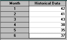
Consider the following example: the demand for a product for 6 months is shown below - calculate the three month moving average for each month and forecast the demand for month 7.
Month             1  2  3  4  5  6
Demand (100's)   42 41 43 38 35 37
Now we cannot calculate a three month moving average until we have at least 3 observations - i.e. it is only possible to calculate such an average from month 3 onward. The moving average for month 3 is given by:
m3 = (42 + 41 + 43)/3 = 42
and the moving average for the other months is given by:
m4 = (41 + 43 + 38)/3 = 40.7
m5 = (43 + 38 + 35)/3 = 38.7
m6 = (38 + 35 + 37)/3 = 36.7
We use m6 as the forecast for month 7. Hence the demand forecast for month 7 is 3670 units.
The package input for this problem is shown below.
The output from the package for a three month moving average is shown below.
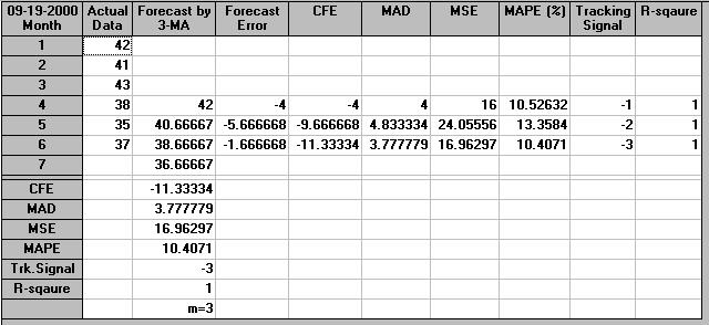
One problem with this forecast is simple - how good is it? For example we could also produce a demand forecast for month 7 using a two month moving average. This would give the following:
m2 = (42 + 41)/2 = 41.5
m3 = (41 + 43)/2 = 42
m4 = (43 + 38)/2 = 40.5
m5 = (38 + 35)/2 = 36.5
m6 = (35 + 37)/2 = 36
Would this forecast (m6 = 3600 units) be better than our current demand forecast of 3670 units?
Rather than attempt to guess which forecast is better we can approach the problem logically. In fact, as will become apparent below, we already have sufficient information to make a logical choice between forecasts if we look at that information appropriately.
In an attempt to decide how good a forecast is we have the following logic. Consider the three month moving average given above and pretend for a moment that we had only demand data for the first three months, then we would calculate the moving average for month 3 (m3) as 42 (see above). This would be our forecast for month 4. But in month 4 the outcome is actually 38, so we have a difference (error) defined by:
Note here that we could equally well define error as outcome-forecast. That would just change the sign of the errors, not their absolute values. Indeed note here that if you inspect the package output you will see that it does just that.
In month 4 we have a forecast for month 5 of m4 = 40.7 but an outcome for month 5 of 35 leading to an error of 40.7-35 = 5.7.
In month 5 we have a forecast for month 6 of m5 = 38.7 but an outcome for month 6 of 37 leading to an error of 38.7-37 = 1.7.
Hence we can construct the table below:
Month             1     2    3    4    5    6    7
Demand (100's)    42    41   43   38   35   37   ?
Forecast          -     -    -    m3   m4    m5   m6
                  -     -    -    42   40.7 38.7 36.7
Error             -     -    -    4    5.7  1.7  ?
Constructing the same table for the two month moving average we have:
Month             1     2    3    4    5    6    7
Demand (100's)    42    41   43   38   35   37   ?
Forecast          -     -    m2   m3    m4   m5   m6
                  -     -    41.5 42   40.5 36.5 36
Error             -     -    -1.5 4    5.5  -0.5 ?
Comparing these two tables we can see that the error terms give us a measure of how good the forecasting methods (two or three month moving average) would have been had we used them to forecast one period (month) ahead on the historical data that we have.
In an ideal world we would like a forecasting method for which all the errors are zero, this would give us confidence (probably a lot of confidence) that our forecast for month 7 is likely to be correct. Plainly, in the real world, we are hardly likely to get a situation where all the errors are zero. It is genuinely difficult to look at (as in this case) two series of error terms and compare them. It is much easier if we take some function of the error terms, i.e. reduce each series to a single (easily grasped) number. One suitable function for deciding how accurate a forecasting method has been is:
The logic here is that by squaring errors we remove the sign (+ or -) and discriminate against large errors (being resigned to small errors but being adverse to large errors). Ideally average squared error should be zero (i.e. a perfect forecast). In any event we prefer the forecasting method that gives the lowest average squared error.
We have that for the three month moving average:
and for the two month moving average:
The lower of these two figures is associated with the two month moving average and so we prefer that forecasting method (and hence prefer the forecast of 3600 for month 7 produced by the two month moving average).
Average squared error is known technically as the mean squared deviation (MSD) or mean squared error (MSE).
Note here that we have actually done more than distinguish between two different forecasts (i.e. between two month and three month moving average). We now have a criteria for distinguishing between forecasts, however they are generated - namely we prefer the forecast generated by the technique with the lowest MSD (historically the most accurate forecasting technique on the data had we applied it consistently across time).
This is important as we know that even our simple package contains many different methods for time series forecasting - as below.
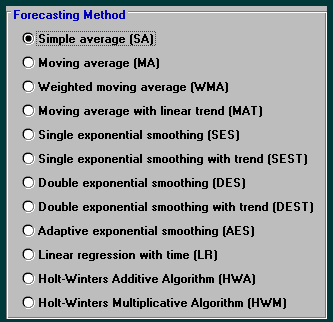
Question - do you think that one of the above forecasting methods ALWAYS gives better results than the others or not?
One disadvantage of using moving averages for forecasting is that in calculating the average all the observations are given equal weight (namely 1/L), whereas we would expect the more recent observations to be a better indicator of the future (and accordingly ought to be given greater weight). Also in moving averages we only use recent observations, perhaps we should take into account all previous observations.
One technique known as exponential smoothing (or, more accurately, single exponential smoothing) gives greater weight to more recent observations and takes into account all previous observations.
Define a constant µ where 0 <= µ <= 1 then the (single) exponentially smoothed moving average for period t (Mt say) is given by
Mt = µYt + µ(1- µ)Yt-1 + µ(1- µ)²Yt-2 + µ(1- µ)³Yt-3 + ...
So you can see here that the exponentially smoothed moving average takes into account all of the previous observations, compare the moving average above where only a few of the previous observations were taken into account.
The above equation is difficult to use numerically but note that:
Mt = µYt + (1- µ)[µYt-1 + µ(1- µ)Yt-2 + µ(1- µ)²Yt-3 + ...]
i.e. Mt = µYt + (1- µ)Mt-1
Hence the exponentially smoothed moving average for period t is a linear combination of the current value (Yt) and the previous exponentially smoothed moving average (Mt-1).
The constant µ is called the smoothing constant and the value of µ reflects the weight given to the current observation (Yt) in calculating the exponentially smoothed moving average Mt for period t (which is the forecast for period t+1). For example if µ = 0.2 then this indicates that 20% of the weight in generating forecasts is assigned to the most recent observation and the remaining 80% to previous observations.
Note here that Mt = µYt + (1- µ)Mt-1 can also be written Mt = Mt-1 - µ(Mt-1 - Yt) or current forecast = previous forecast - µ(error in previous forecast) so exponential smoothing can be viewed as a forecast continually updated by the forecast error just made.
Consider the following example: for the demand data given in the previous section calculate the exponentially smoothed moving average for values of the smoothing constant µ = 0.2 and 0.9. We have the following for µ = 0.2.
M1 = Y1 = 42 (we always start with M1
= Y1)
M2 = 0.2Y2 + 0.8M1 = 0.2(41) + 0.8(42)
= 41.80
M3 = 0.2Y3 + 0.8M2 = 0.2(43) + 0.8(41.80)
= 42.04
M4 = 0.2Y4 + 0.8M3 = 0.2(38) + 0.8(42.04)
= 41.23
M5 = 0.2Y5 + 0.8M4 = 0.2(35) + 0.8(41.23)
= 39.98
M6 = 0.2Y6 + 0.8M5 = 0.2(37) + 0.8(39.98)
= 39.38
Note here that it is usually sufficient to just work to two or three decimal places when doing exponential smoothing. We use M6 as the forecast for month 7, i.e. the forecast for month 7 is 3938 units.
We have the following for µ = 0.9.
M1 = Y1 = 42
M2 = 0.9Y2 + 0.1M1 = 0.9(41) + 0.1(42)
= 41.10
M3 = 0.9Y3 + 0.1M2 = 0.9(43) + 0.1(41.10)
= 42.81
M4 = 0.9Y4 + 0.1M3 = 0.9(38) + 0.1(42.81)
= 38.48
M5 = 0.9Y5 + 0.1M4 = 0.9(35) + 0.1(38.48)
= 35.35
M6 = 0.9Y6 + 0.1M5 = 0.9(37) + 0.1(35.35)
= 36.84
As before M6 is the forecast for month 7, i.e. 3684 units.
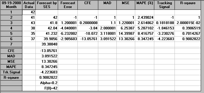
The package output for µ=0.2 is shown below.
The package output for µ=0.9 is shown below.

In order to decide the best value of µ (from the two values of 0.2 and 0.9 considered) we choose the value associated with the lowest MSD (as above for moving averages).
For µ=0.2 we have that
For µ=0.9 we have that
Note here that these MSD values agree (to within rounding errors) with the MSD values given in the package output above.
Hence, in this case, µ=0.9 appears to give better forecasts than µ=0.2 as it has a smaller value of MSD.
Above we used MSD to reduce a series of error terms to an easily grasped single number. In fact functions other than MSD such as:
and
exist which can also be used to reduce a series of error terms to a single number so as to judge how good a forecast is.
For example, as can be seen in the package outputs above, the package gives a number of such functions, defined as:

In fact methods are available which enable the optimal value of the smoothing constant (i.e. the value of µ which minimises the chosen criteria of forecast accuracy, such as mean squared deviation (MSD)) to be easily determined. This can be seen below where the package has calculated that the value of µ which minimises MSD is µ=0.86 (approximately).

Note here that the package can be used to plot both the data and the forecasts as generated by the method chosen. Below we show this for the output above (associated with the value of µ which minimises MSD of 0.86.
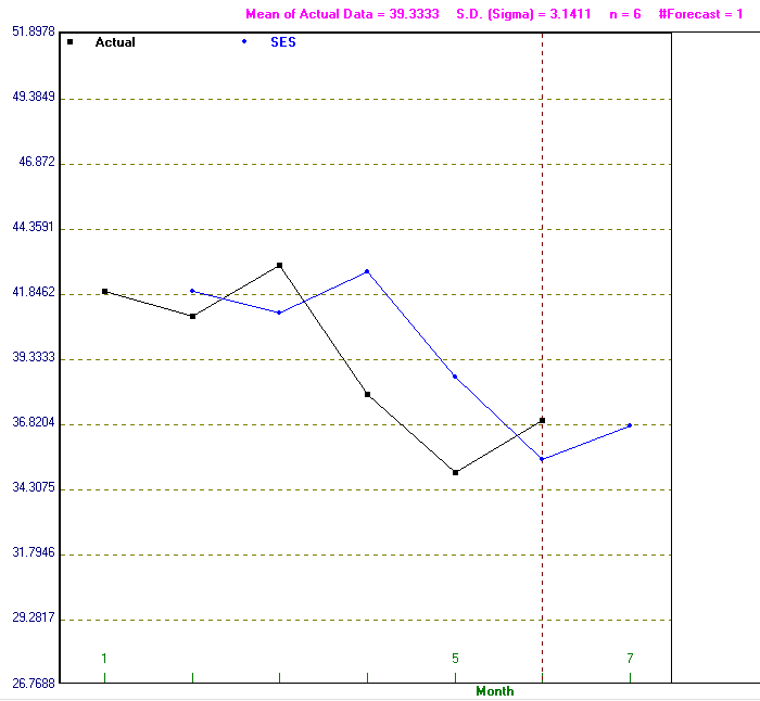
Note here that the choice of criterion can have a large effect on the value of µ e.g. for our example the value of µ which minimises MAD is µ=0.59 (approximately) and the value of µ which minimises bias is µ=1.0 (approximately).
To illustrate the change in MAD, bias and MSD as µ changes we graph below MAD and bias against the smoothing constant µ,
and below MSD against µ.
Below we graph the value of the forecast against µ. One particular point to note is that, for this example, for a relatively wide range of values for µ the forecast is stable (e.g. for 0.60 <= µ <= 1.00 the forecast lies between 36.75 and 37.00). This can be seen below - the curve is "flat" for high µ values.
Note here that the above graphs imply that in finding a good value for the smoothing constant it is not usually necessary to calculate to a very high degree of accuracy (e.g. not to within 0.001 for example).
Time series forecasting methods more advanced than those considered in our simple package do exist. These are based on AutoRegressive Integrated Moving Average (ARIMA) models. Essentially these assume that the time series has been generated by a probability process with future values related to past values, as well as to past forecast errors. To apply ARIMA models the time series needs to be stationary. A stationary time series is one whose statistical properties such as mean, variance and autocorrelation are constant over time. If the initial time series is not stationary it may be that some function of the time series, e.g. taking the differences between successive values, is stationary.
In fitting an ARIMA model to time series data the framework usually used is a Box-Jenkins approach. It does however have the disadvantage that whereas a number of time series techniques are fully automatic, in the sense that the forecaster has to exercise no judgement other than in choosing the technique to use, the Box-Jenkins technique requires the forecaster to make judgements and consequently its use requires experience and "expert judgement" on the part of the forecaster. Some forecasting packages do exist that make these "expert choices" for you.
More about ARIMA and Box-Jenkins can be found here, here and here.
We have given just an overview of the types of forecasting methods available. The key in forecasting nowadays is to understand the different forecasting methods and their relative merits and so be able to choose which method to apply in a particular situation (for example consider how many time series forecasting methods the package has available).
All forecasting methods involve tedious repetitive calculations and so are ideally suited to be done by a computer. Forecasting packages, many of an interactive kind (for use on pc's) are available to the forecaster.
Some more forecasting examples can be found here.