OR-Notes are a series of introductory notes on topics that fall under the broad heading of the field of operations research (OR). They were originally used by me in an introductory OR course I give at Imperial College. They are now available for use by any students and teachers interested in OR subject to the following conditions.
A full list of the topics available in OR-Notes can be found here.
In many problems chance (or probability) plays an important role. Decision analysis is the general name that is given to techniques for analysing problems containing risk/uncertainty/probabilities. Decision trees are one specific decision analysis technique and we will illustrate the technique by use of an example.
A company faces a decision with respect to a product (codenamed M997) developed by one of its research laboratories. It has to decide whether to proceed to test market M997 or whether to drop it completely. It is estimated that test marketing will cost £100K. Past experience indicates that only 30% of products are successful in test market.
If M997 is successful at the test market stage then the company faces a further decision relating to the size of plant to set up to produce M997. A small plant will cost £150K to build and produce 2000 units a year whilst a large plant will cost £250K to build but produce 4000 units a year.
The marketing department have estimated that there is a 40% chance that the competition will respond with a similar product and that the price per unit sold (in £) will be as follows (assuming all production sold):
                                         Large plant     Small plant
Competition respond                      20              35
Competition do not respond               50              65
Assuming that the life of the market for M997 is estimated to be 7 years and that the yearly plant running costs are £50K (both sizes of plant - to make the numbers easier!) should the company go ahead and test market M997?
Although the above example is somewhat simplified it plainly represents the type of decision that often has to be made about new products.
In particular note how we cannot separate the test market decision from any decisions about the future profitability (if any) of the product if test marketing is successful.
To enable us to see what is going on consider the figure below where we have drawn the decision tree for the problem.
In that figure we have three types of node represented:
Decision nodes represent points at which the company has to make a choice of one alternative from a number of possible alternatives e.g. at the first decision node the company has to choose one of the two alternatives "drop M997" or "test market M997".
Chance nodes represent points at which chance, or probability, plays a dominant role and reflect alternatives over which the company has (effectively) no control.
Terminal nodes represent the ends of paths from left to right through the decision tree.
It is worth saying here that the difficult part of the decision tree technique is drawing up a diagram such as the figure above from the written description of the problem. Once that has been done the solution procedure is quite straightforward. Note here that most, but not all, decision trees start with a decision node. One tip that may help you to draw decision trees is to ask yourself the question "What happens next?" at each point in the tree as you draw it.
Note here the inclusion of the "no plant" alternative at the plant size decision node. This is necessary because it simply may not be profitable to build any plant (large or small) even if the product is successful in test market. It is common in decision tree problems to find that at decision nodes we need a "do nothing" alternative which is an implicit decision that can be taken.
Note that it is important for the decision tree to be drawn so that there is a unique path in the tree from the initial node to each of the terminal nodes.
To ease the discussion of the decision tree we have numbered the nodes (decision/chance/terminal) 1,2,3,...,12. At each decision node we have also numbered the alternatives, at node 1 we have alternatives 1 and 2 and at node 5 alternatives 3, 4 and 5.
Although the decision tree diagram does help us to see more clearly the nature of the problem it has not, so far, helped us to decide whether to drop M997 or whether to test market it (the decision we are trying to make!). To do this we have two steps as illustrated below.
In these steps we will need to use information (numbers) relating to future sales, prices, costs, etc. Whilst we may not be able to give accurate figures for these we need to factor such figures into our calculations if we are to proceed. Investigating how our decision to test market or not might change as these figures change (i.e. sensitivity analysis) can be done once we have carried out the basic calculations using our assumed figures.
In this step we, for each path through the decision tree from the initial node to a terminal node of a branch, work out the profit (in £) involved in that path. Essentially in this step we work from the left-hand side of the diagram to the right-hand side.
Total revenue = 0
Total cost = 0
Total profit = 0
Note that we ignore here (and below) any money already spent on developing M997 (that being a sunk cost, i.e. a cost that cannot be altered no matter what our future decisions are, so logically has no part to play in deciding future decisions).
Total revenue = 0
Total cost = 100
Total profit = -100 (all figures in £K)
Total revenue = 910
Total cost = 250 + 7x50 (running cost)
Total profit = 310
Total revenue = 490
Total cost = 250 + 7x50
Total profit = -110
Total revenue = 1400
Total cost = 350 + 7x50
Total profit = 700
Total revenue = 560
Total cost = 350 + 7x50
Total profit = -140
Total revenue = 0
Total cost = 100
Total profit = -100
Note that, as mentioned previously, we include this option because, even if the product is successful in test market, we may not be able to make sufficient revenue from it to cover any plant construction and running costs.
Hence we can form the table below indicating, for each branch, the total profit involved in that branch from the initial node to the terminal node.
Terminal node                Total profit (£K)
        2                          0
        4                       -100
        7                        310
        8                       -110
        10                       700
        11                      -140
        12                      -100
So far we have not made use of the probabilities in the problem - this we do in the second step where we work from the right-hand side of the diagram back to the left-hand side.
Consider chance node 6 with branches to terminal nodes 7 and 8 emanating from it. The branch to terminal node 7 occurs with probability 0.6 and total profit 310K whilst the branch to terminal node 8 occurs with probability 0.4 and total profit -110K. Hence the expected monetary value (EMV) of this chance node is given by
0.6 x (310) + 0.4 x (-110) = 142 (£K)
Essentially this figure represents the expected (or average) profit from this chance node (60% of the time we get £310K and 40% of the time we get -£110K so on average we get (0.6 x (310) + 0.4 x (-110)) = 142 (£K)).
The EMV for any chance node is defined by "sum over all branches, the probability of the branch multiplied by the monetary (£) value of the branch". Hence the EMV for chance node 9 with branches to terminal nodes 10 and 11 emanating from it is given by
0.6 x (700) + 0.4 x (-140) = 364 (£K)
node 10       node 11
We can now picture the decision node relating to the size of plant to build as below where the chance nodes have been replaced by their corresponding EMV's.
Hence at the plant decision node we have the three alternatives:
Alternative 3: build small plant EMV = 142K
Alternative 4: build large plant EMV = 364K
Alternative 5: build no plant EMV = -100K
It is clear that, in £ terms, alternative number 4 is the most attractive alternative and so we can discard the other two alternatives, giving the revised decision tree shown below.
We can now repeat the process we carried out above.
The EMV for chance node 3 representing whether M997 is a success in test market or not is given by
0.3 x (364)         +  0.7 x (-100) = 39.2 (£K)
plant decision node    node 4
Hence at the decision node representing whether to test market M997 or not we have the two alternatives:
Alternative 1: drop M997 EMV = 0
Alternative 2: test market M997 EMV = 39.2K
It is clear that, in £ terms, alternative number 2 is preferable and so we should decide to test market M997.
Let us be clear then about what we have decided as a result of the above process:
Note here that the EMV of our decision (39.2 in this case) DOES NOT reflect what will actually happen - it is merely an average or expected value if we were to have the tree many times - but if fact we have the tree once only. If we follow the path suggested above of test marketing M997 then the actual monetary outcome will be one of [-100, 310, -110, 700, -140, -100] corresponding to terminal nodes 4,7,8,10,11 and 12 depending upon future decisions and chance events.
Conceptually one can think of the set of terminal nodes that can be reached as a result of our test market decision as the set of possible futures. The best possible future corresponding to the decision to test market M997 is called the upside and the worst possible future corresponding to the decision to test market M997 is called the downside.
We need to be slightly careful here since, as noted above, the actual monetary outcomes will depend both upon future decisions and chance events.
If we are committed to a large plant (assuming we are successful in test market) then the set of possible futures is given by [-100, 700, -140] corresponding to terminal nodes 4,10 and 11 and hence the upside is 700 (£K) and the downside is -140 (£K).
If we are not committed to a large plant (assuming we are successful in test market) then the set of possible futures is given by [-100, 310, -110, 700, -140, -100] corresponding to terminal nodes 4,7,8,10,11 and 12 and hence the upside is 700 (£K) and the downside is -140 (£K).
Whilst in this particular example the upside and downside are the same irrespective of whether we are committed to a large plant or not note how the possible futures are different depending upon whether we are committed to a large plant or not.
The above problem was solved using the package, the input being shown below. The description of the input is as follows. All data is entered by nodes in the tree. Each node has a type (d for decision nodes and c for chance nodes), or is left blank for terminal nodes. All following nodes in the decision tree are listed.
If a node comes from a chance node then it has a non-zero probability value assigned. If the node is a terminal node then a payoff/cost is also assigned.

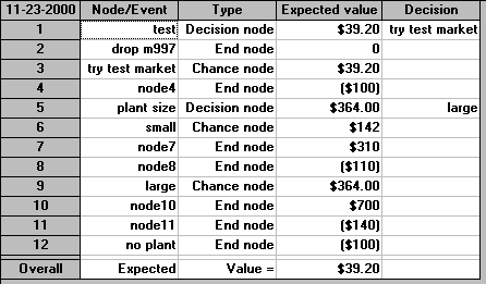
In the output shown below we have for each decision node the expected value and the appropriate decision and for each chance node the expected value.

It is clear that the package agrees with the calculation we carried out
before.
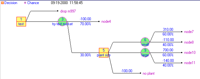
Note here that this package is also capable of drawing the tree for use from the input, so we can check we have entered it correctly), as below.

Note here that since the decision tree calculation is so straightforward it is relatively easy to conduct sensitivity analysis to see how the recommended course of action changes (if at all) in response to data changes.
Consider the decision tree given above. It is plain that the decision to test market is influenced by the profit of 700 (£K) that we will get if test marketing is successful and we choose to build a large plant and we find that we have no competition. Colloquially we could say that we are "following the money". Hence we may vary this figure of 700 (and/or vary the probability that this outcome occurs) to see if it changes the test market decision.
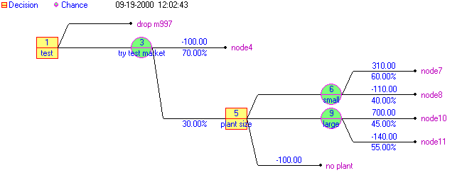
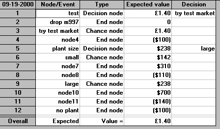
For example, suppose the probability that we have no competition with a large plant is no longer 0.6 but is instead 0.45. This implies that the probability that we have competition is hence 1-0.45=0.55. Redoing the decision tree calculation (here using the package) we get:


Hence we can see that the initial decision (to test market) is still the optimal decision.
We can also conduct sensitivity analysis using a more systematic algebraic basis (i.e. assign a symbol p to a given probability and work out algebraic expressions for EMVs). To see this suppose that the probability of competition with a large plant is no longer 0.6 but is instead p. This implies that the probability that we have competition is hence 1-p. Assume that we can leave the probabilities for a small plant of competition/no competition unaltered. It is clear that as p decreases we will at some stage prefer a small plant over a large plant (e.g. if p=0 then a small plant with EMV of 142 would be preferable to a large plant with EMV of -140). We can therefore ask the logical question "How small does p have to be before we prefer a small plant?"
To answer this question we have that we will be indifferent between a small and a large plant when their EMVs are equal, i.e. when
p(700) + (1-p)(-140) = 142
i.e. when 840p - 140 = 142, so p = 282/840 = 0.3357
Hence if p drops below 0.3357 we would prefer a small plant to a large plant. This type of systematic sensitivity analysis can be preferable in some circumstances to simply trying different numbers and redoing the calculation to see what the effect is.
The basic decision tree technique presented above can be applied to any problem for which a decision tree can be drawn. There are a number of extensions to the technique and we briefly consider four such extensions below. These relate to:
We consider each in turn.
In the example given above we were concerned with money received over 7 years. It is plain that £1 received in seven years time is worth less than £1 received now and a technique called discounting, or discounted cash flow, (involving finding the net present value of any sum of money) can be used to overcome this difficulty. Applying discounting merely alters the numbers which are fed into the decision tree so that we are dealing with monetary values on an equivalent (present-day) basis. It does not effect the processing of the tree (which remains exactly as indicated above).
In the example given above we calculated a value for each chance node. Whilst we have used EMV as the value of a chance node this choice is, in many respects, somewhat arbitrary and other ways of calculating a value for a chance node have been suggested. To put it another way whilst it is a law of the universe (in this particular corner of the space-time continuum) that E=mc2 it is not a law of the universe that the value of a chance node must be the equal to the EMV value!
Reflect that EMV is an average value - but at a chance node we never see the average - something happens once only (e.g. at chance node 6 we either see competition or not). Hence perhaps the average value is misleading and we need to look at a chance node a different way.
If we were adverse to losing money and wished to take a conservative attitude to decision making (risk) we might calculate the value of a chance node as the worst possible outcome that might occur at that node. Such a strategy is often called a pessimistic strategy (e.g. such a strategy would assign chance node 6 a value of -110 compared with an EMV of 142).
An alternative strategy would be the optimistic strategy of calculating the value of a chance node as the best possible outcome that might occur at that node (e.g. such a strategy would assign chance node 6 a value of 310 compared with an EMV of 142).
Yet another strategy would be to take the value of a chance node as equal to the most likely (highest probability) outcome that might occur at that node (e.g. such a strategy would assign chance node 4 a value of 310 compared with an EMV of 142).
Alternatively we might take the value of a chance node to be some weighted combination of the EMV and the values given by the optimistic and pessimistic strategies. The literature contains a number of variations on this theme of changing the value of a chance node.
At each decision node we choose one of the alternative decisions at that node based upon an implicit rule ("choose the alternative with the highest EMV"). Other rules are equally plausible (e.g. "choose the alternative with the highest ROI" (ROI = return on investment = profit divided by total investment)).
For example consider the small and large plants above. We saw that a small plant led to an EMV (actually an expected net profit) of 142. That involved a total investment of 100 for test marketing plus 150 to build, so a ROI of 142/(100+150) = 56.8%
A large plant led to an EMV (actually an expected net profit) of 364. That involved a total investment of 100 for test marketing plus 250 to build, so a ROI of 364/(100+250) = 104%
Whilst, in this case ROI would lead to the same decision relating to the size of plant to build it could have led to a different decision. For example had the EMV at chance node 9 been 175 then on an EMV basis we would still have chosen at decision node 5 to build a large plant. But on a ROI basis [175/(100+250) = 50%] we would chose to build a small plant.
Using monetary values in the decision tree implies, for example, that a loss of 200K is only twice as bad as a loss of 100K. If the company doesn't have 200K to lose, but does have 100K, then it is plain that they will regard losing 200K as much worse than losing 100K. Moreover note that often decisions are made by people within the company. The company makes the profit/loss, not the people concerned with the decision.
Hence the idea of utility is to replace the monetary values at each terminal node in the decision tree by utilities (points) which reflect the view of the decision maker (or company) to that sum of money (e.g. a loss of 100K might get a utility value of -5 but a loss of 200K a utility value of -500). In simple terms you can think of utilities as replacing £'s by points.
Trying to capture the decision-maker's translation of £'s to points is an imprecise process, but it does enable the decision-maker's valid view of the problem in terms of the importance of £'s to them to be incorporated. Once utility values have been found then we proceed as before.
Some more decision tree examples can be found here.