Bioinformatics - Lab 9
Biochemical Pathways
David Gilbert and Xu Gu
The purpose of this lab is to give you practical experience in the
construction and simulation of models of biochemical networks.
This lab refers to the slides for the lecture on Modelling dynamic behaviour.
Software
Matlab:
- Matlab is a modelling and simulation language that encourages the
experimentation of system biology models. In Matlab, models of
biochemical pathways are written as functions (M files), which are then solved with differential equations solvers (e.g. ode15 and ode45).
- Matlab can be run at any local machine.
BioNessie:
- BioNessie http://www.bionessie.com is a
software tool which allows users to compose models of biochemical
systems using biochemical equations, and to save these models as in
SBML format (see http://www.sbml.org
for model details on SBML---basically, it is a mark-up language for
biochemical models).
- BioNessie enables the simulation of dynamic behaviour of
biochemical models using a differential equation solver, and displays
the results graphically. It also supports advanced analysis methods,
including parameter scans and sensitivity analysis.
- BioNessie is available at
/local/brccontrib/bin/bpi. For more information about
using BioNessie, please see the user
manual.
Exercises 1
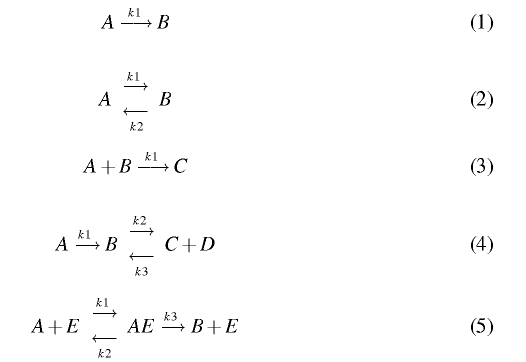
Use BioNessie and Matlab to create a Mass Action
based computational model for each of the following biochemical
descriptions and produce simulations for each of the models. You
should be able to check by eye how similar the simulation results are.
Descriptions
Rate constants and initial concentrations required for the
simulation are:
- Rate Constants: k1 = 1; k2 = 0.5; k3 = 2
- Initial Concentrations: [A] = 5; [B] = 1; [C] = 0; [D] = 0;
[E] = 1; [AE]= 0;

See slides
variable from the lecture notes for the Matlab code of
equation (1) and equation (2) respectively. Click here to see how to create
models in Matlab.
Exercise 2
(A) With the experience of modelling equation(5), can you code
and simulate (i) a Metabolic Pathway and (ii) Signalling
Pathway in BioNessie? See slides
variable from the lecture notes for more details of the pathways. Refer to the following information to model and simulate the pathways.
- Rate constants are the same as that in equation (5).
- Initial concentrations of all enzyme-substrate complexes are given to 0.
- Initial concentrations of substrates, products and enzymes
involved in these two pathways are:
- Metabolic Pathway: [E1] = [E2] = [E3] = 1; [S] = 100; [S'] = [S''] = [S'''] = 0
- Signalling Pathway: [Input Signal] = 1; [S1] = [S2] = [S3] = 100;
[P1] = [P2] = [P3] = 0
(B) Model and simulate the above pathways in Matlab. Can you tell
the difference in the usability of command-line based simulator and
equation-based simulator?
Exercise 3
Use BioNessie to perform a simulation and advanced analysis of the
model of Raf-1/RKIP/ERK pathway. Click here to view the topology of
the pathway. An available SBML model of the pathway can be
downloaded here
(right click on the link and save it with the name RKIP.xml).
(A) Run a time-plot simulation of the model (RKIP.xml) in
BioNessie. Refer to the user
manual for uploading SBML files with BioNessie.
(B) Perform parameter scans and sensitivity analysis of the SBML
model (RKIP.xml). Parameter scans and sensitivity
analysis are two commonly used approaches for understanding
the dynamics of a biochemical model. Basically, parameter scanning is
to explore a model's behaviour over different ranges of parameter
values, which is achieved by running simulations for specific values in
the range. Sensitivity analysis is to study the response of system
variables to changes in parameter values, which can be used to
identify key reactions and species as well as monitoring the robustness
of a model.
- Perform a standard parameter scan for k2 over the range of values
between 0 and 5 with the settings below. Go to the user manual for
running a parameter scan in BioNessie.
- Param Scan Option = k2
- Param Begin value = 0; Param End Value = 5
- Param Steps = 10
- Total time = 200; Time step = 200
- Perform a monitoring-function based parameter scan for k2 with the
same settings as defined above. In addition to view changes in dynamics
of each individual species over a range of parameter values, you can
also examine the response of some particular targets by defining
corresponding monitoring functions. Go to the user manual for
running a monitoring-function based parameter scan.
In this exercise, you will use BioNessie to run two
monitoring-function based parameter scans:
- Monitoring function: ERK + RKIP. The function examines the effect
of k2 on the total concentration of ERK and RKIP.
- Monitoring function: MEKPP * RP. The function examines the effect
of k2 on the production of the concentrations of MEKPP and RP.
- Perform a sensitivity analysis for the parameter k6 with the following settings. Go to the user manual for
running a sensitivity analysis in BioNessie.
- Total time = 200; Time steps = 200
The page was last modified on 11th March 2007.
